Machine Learning (Coursera, Andrew Ng)

Some notes I took while taking Machine Learning taught by Andrew Ng on Coursera.

BTW, if you also choose to use Python to do the homework assignments rather than Octave/Matlab, this tool made by dibgerge will save your life. You can now get the credit while coding in Python!!!

Week 1 - Introduction, Linear Regression with One Variable, Linear Algebra Review

Definitions of Machine Learning

Arthur Samuel (1959):
ML is the field of study that gives computers the ability to learn without being explicitly learned.

Tom Mitchell (1998):
A computer program is said to learn from experience E with respect to some task T and some performance measure P, if its performance on T, as measured by P, improves with experience E.

Types of Machine Learning Algorithms

• Supervised learning:
  • teach computers
  • “right answer” is given
  • types of problems: regression (continued valued output e.g. housing price), classification (discrete-valued output e.g. malignant or benign tumor)
• Unsupervised learning:
  • let the computers learn by themselves
  • no “right answer” is given
  • a similar example as the tumor example: same points, but instead of blue circles and red crosses, they are not labeled at all
  • types of problems: clustering (e.g. cluster the two groups of points in the given dataset)

Model Representation

We feed the training set (a group of $(x,y)$’s) to the learning algorithm, and it will produce a hypothesis h (“hypothesis” is the term in ML for a function that does the following mapping). $h$ will map from $x$ to $y$, where $x$ is the known and the $y$ is the result we want (e.g. $x$ is the area of the house and $y$ is the price it worth)

e.g. (univariate) linear regression: $h(x) = \theta_0 + \theta_1 x$

Our goal for linear regression: minimize the cost function (aka square error function)

$$J(\theta_0, \theta_1) = \frac{1}{2m}\sum_{i=1}^{m} (h(x_i) - y_i)^2$$

where $m$ is the size of the training set.

$h$ is a function of $x$, and $J$ is a function of $\theta_0$ and $\theta_1$.

Gradient Descent

$$\min_{\theta_0, \theta_1, \ldots, \theta_n} J(\theta_0, \theta_1, \ldots, \theta_n)$$

Outline:

• Start with some $\theta_i$’s
• Keep changing their value to reduce the value of the cost function
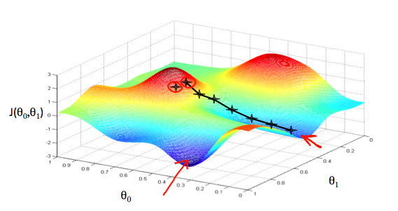
• Imagine: taking one little step from the current point to get as low as possible, and start over again from the new point we stand at - $\theta_0 := \theta_0 - \alpha \frac{\partial}{\partial \theta_0}J(\theta_0, \theta_1)$ and $\theta_1 := \theta_1 - \alpha \frac{\partial}{\partial \theta_1}J(\theta_0, \theta_1)$, where $\alpha$ is the learning rate (the length of each step)
• The updates to each $\theta_j$ should be simultaneous
• As we approach local minimum, gradient descent will automatically take smaller steps, since the derivatives are closer to 0. And when we finally reach the local minimum, the derivative term will be 0, so we won’t move anymore

Week 2 - Linear Regression with Multiple Variables

Multivariate Linear Regression

Gradient Descent for multiply variables:

$$\theta_j := \theta_j - \alpha \frac{\partial}{\partial \theta_j}J(\theta)$$

i.e.

$$\theta_j := \theta_j - \alpha \frac{1}{m}\sum_{i=1}^{m} (h(x^{(i)}) - y^{(i)})x_j^{(i)}$$

for $j \in {0, 1, \ldots, n}$.

Feature Scaling

Ideas:

1. Make sure the features are on a similar scale
   • e.g. if the contour is of a skewed elliptical shape, gradient descent may take a lot of back and forth (zigzag) steps before reaching the global minimum. However, if we scale the variables, the contour will look much less skewed (like circles in our example), and gradient descent will take less time.
2. Get every feature into approximately a $-1 \leq x_i \leq 1$ range

Mean Normalization

Replace $x_i$ with $x_i - \mu_i$ to make features have approximately 0 mean (doesn’t apply to $x_0 = 1$)

In a word, replace $x_i$ with $x_i = \frac{x_i - \mu_i}{s_i}$, where $\mu_i$ is the mean of the feature and $s_i$ is the range (max - min) of the feature

Make sure gradient descent is working:

If $J(\theta)$ increases after each iteration, we may consider choosing a smaller learning rate $\alpha$.

• For sufficiently small $\alpha$, $J(\theta)$ should decrease on every iteration.
• But if $\alpha$ is too small, gradient descent can be slow to converge.

Polynomial Regression

Feature scaling is very important!

e.g. size ranges from 1 to 1000, then the square of it will range from 1 to 1,000,000 and so on.

Normal Equation

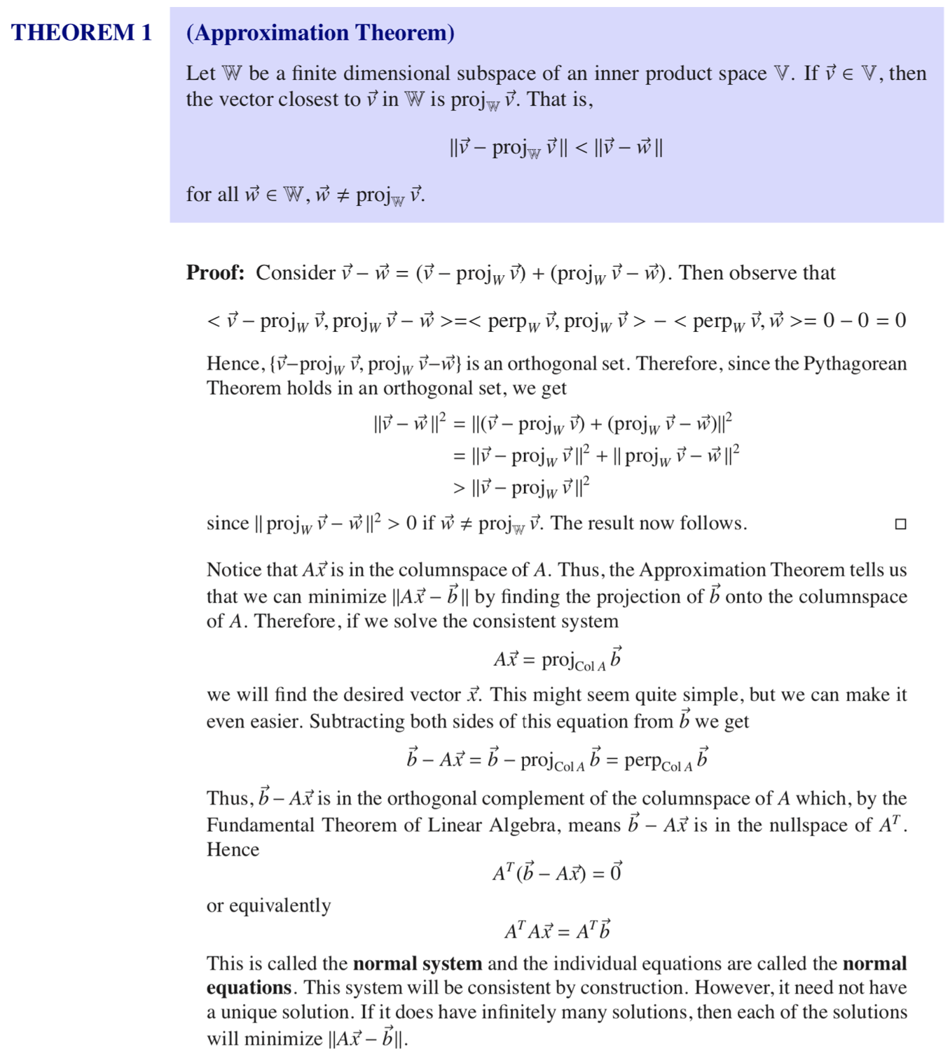
Instead of using gradient descent and run many iterations, we can also calculate the partial derivations of each $\theta_i$ and let the derivations to be zero. The values of the $\theta_i$’s when the derivations are zero will be the values we want.

How to find the values of the $\theta_i$’s?

(Andrew Ng doesn’t cover this part, so I copied from Linear Algebra 2 Course Notes for MATH 235 by Dan Wolczuk from UWaterloo)

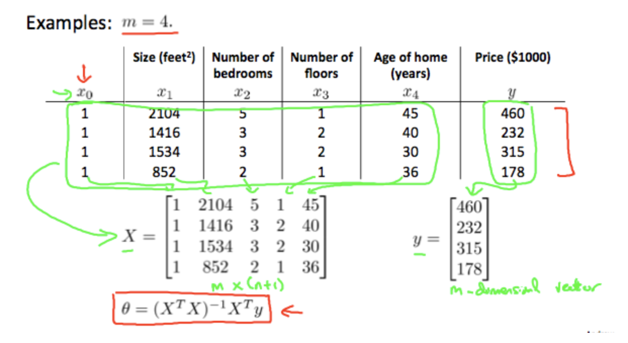
==If we’re using the normal equation method, then feature scaling isn’t necessary.==

When to use what?

Normal equation works well when $n$ is small (say, < 1000). However, for some more complicated algorithms, normal equation doesn’t work — we still need gradient descent for those algorithms.

But for linear regression, normal equation is a great alternative. Sometimes it can be much faster than gradient descent.

Normal Equation Noninvertibility

The reasons why $X^TX$ can be non-invertible could be:

• redundant features (linearly dependent, e.g. one feature is the size and another feature is size * 2)
• too many features (e.g. m <= n)

Week 3 - Logistic Regression, Regularization

Classification Problems

Applying linear regression to a classification problem often isn’t a great idea.

Some reasons (we’re talking about binary classification problems):

• recall the example when we add a new point to the RHS and the slope of the line changed a bit, hence changed the prediction for some points.
• linear regression can produce values >1 or <0, while we know the results can only be 0 or 1

Therefore, let’s take a look at logistic regression where $0 \leq h(x) \leq 1$.

Sigmoid function / logistic function:
$h(x) = g(\theta^Tx)$ where $g(z) = \frac{1}{1+e^{-z}}$.
That is, $h(x) = \frac{1}{1+e^{-\theta^Tx}}$.

Note that for the sigmoid function, when z < 0, g(z) is close to 0, and when z >= 0, g(z) is close to 1. So according to our definition, if $\theta^Tx < 0$, we say we predict a negative case, while if $\theta^Tx \geq 0$, we predict a positive case.

The boundary we have between the two groups is called the decision boundary.

Cost Function for Logistic Regression

Firstly, why can’t we use the same cost function as in linear regression?

That’s because if we use the same

$$J(\theta) = \frac{1}{2m}\sum_{i=1}^{m} (h(x_i) - y_i)^2$$

as in linear regression, the cost function is non-convex (may not end up at a global minimum). We want a convex bowl-shape cost function so that we can end up at the global minimum.

So instead of using the same cost function as in linear regression, we should come up with a new cost function that is convex for logistic regression.

Logistic regression cost function:

$$\text{Cost}(h_\theta(x), y) = \begin{cases} -\log(h_\theta(x)) \text{ if } y = 1 \\ -\log(1 - h_\theta(x)) \text{ if } y = 0\\ \end{cases}$$

Write in one line:

$$\text{Cost}(h_\theta(x), y) = -y\log(h_\theta(x)) - (1-y)\log(1-h_\theta(x))$$

So

$$J(\theta) = \frac{1}{m}\sum_{i=1}^{m} \text{Cost}(h_\theta(x^{(i)}), y^{(i)}) = -\frac{1}{m}\sum_{i=1}^{m}y^{(i)}\log(h_\theta(x^{(i)})) + (1-y^{(i)})\log(1-h_\theta(x^{(i)}))$$

Again, by taking derivative:

$$\theta_j := \theta_j - \alpha \frac{\partial}{\partial \theta_j}J(\theta)$$

That is,

$$\theta_j := \theta_j - \alpha \frac{1}{m}\sum_{i=1}^{m} (h(x^{(i)}) - y^{(i)})x_j^{(i)}$$

This is exactly the same as what we got for linear regression! That because for linear regression, $h(x) = \theta^Tx$ while for logistic regression, $h(x) = \frac{1}{1+e^{-\theta^Tx}}$

We might use a more advanced optimization algorithm (e.g. conjugate gradient/BFGS/L-BFGS etc) because they can be faster and don’t require a learning rate.

Multiclass classification

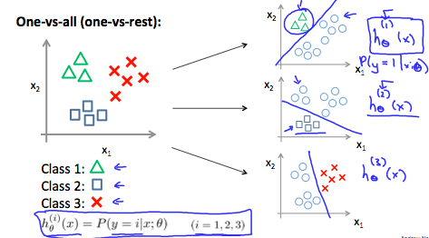
One-vs-all (one-vs-rest): train a logistic regression classifier $h_\theta^{(i)}(x)$ for each class $i$ to predict the probability that $y=i$

The Problem of Overfitting

• Underfitting / High bias
• “Just right”
• Overfitting / High variance

The problem of overfitting: if we have too many features, then the model may fit the training set very well. So, the cost function may actually be very close to zero or maybe even zero exactly, but we may then end up with a very wiggly curve (try too hard to fit the training set), so that it may fail to generalize to new examples.

How to address overfitting?

• Reduce the number of features
• Regularization

Regularization

Intuition:

Suppose an overfitting expression is $\theta0 + \theta_1 x + \theta_2 x^2+ \theta_3 x^3 + \theta_4 x^4$. We know it’s a overfitting, and we want $\theta_3$ and $\theta_4$ to be small - we penalize on $\theta_3$ and $\theta_4$:
Make the cost function to be $\frac{1}{2m}\sum{i=1}^{m} (h(x^{(i)}) - y^{(i)})^2 + 1000\theta_3^2 + 1000\theta_4^2$ and try to minimize this.

This will make $\theta_3$ and $\theta_4$ as close to 0 as possible.

However, if there are many parameters, we don’t which are the ones that should be regularized. In this case, we regularize all the parameters: cost function

$$J(\theta) = \frac{1}{2m}[\sum_{i=1}^{m} (h(x^{(i)}) - y^{(i)})^2 + \lambda\sum_{j=1}^{n} \theta_j^2]$$

where the $\lambda$ is the regularization parameter. It determines how much the costs of our theta parameters are inflated. Also note that for the lambda part, we don’t regularize $\theta_0$.

Gradient Descent when Regularized

So for gradient descent, the unregularized gradient is

$$\frac{\partial J}{\partial \theta_j} = \frac{1}{m}\sum_{i=1}^{m} (h(x^{(i)}) - y^{(i)})x_j^{(i)}$$

The regularized gradient is

$$\frac{\partial J}{\partial \theta_i} = \begin{cases} \frac{1}{m}\sum_{i=1}^{m} (h(x^{(i)}) - y^{(i)})x_0^{(i)} \text{ if } j = 0 \\ \frac{1}{m}\sum_{i=1}^{m} (h(x^{(i)}) - y^{(i)})x_j^{(i)} + \frac{\lambda}{m}\theta_j \text{ if } j > 0\\ \end{cases}$$

We do the simultaneous update:

$$\theta_0 := \theta_0 - \alpha \frac{1}{m}\sum_{i=1}^{m} (h(x^{(i)}) - y^{(i)})x_0^{(i)} \\ \theta_j := \theta_j - \alpha [\frac{1}{m}\sum_{i=1}^{m} (h(x^{(i)}) - y^{(i)})x_j^{(i)} + \frac{\lambda}{m}\theta_j] \\ =\theta_j(1 - \alpha\frac{\lambda}{m}) - \theta_j - \alpha \frac{1}{m}\sum_{i=1}^{m} (h(x^{(i)}) - y^{(i)})x_j^{(i)},\;\forall j = 1, 2, \ldots, n$$

Normal Equation when Regularized

$$\theta = (X^TX + \lambda \begin{bmatrix} 0 & 0 & 0 & \ldots & 0\\ 0 & 1 & 0 & \ldots & 0\\ 0 & 0 & 1 & \ldots & 0\\ 0 & 0 & 0 & \ldots & 0\\ 0 & 0 & 0 & \ldots & 1\end{bmatrix})^{-1} X^Ty$$

The matrix is a $(n+1) * (n+1)$ matrix, and all diagonal entries except for the top left corner is 1.

Week 4 - Neural Networks: Representation

Non-linear Hypotheses

Why do we need yet another learning algorithm? We already have linear regression and we have logistic regression, so why do we need neural networks?

That’s because when the number of features is large, the computation will be very hard.

For example, if there are $n$ features $x_1, x_2, \ldots, x_n$, and we want to include all the quadratic terms, there would be terms like $x_1^2, x_1x_2, x_1x_3, \ldots, x_2^2, x_2x_3, \ldots$. That’s about $n^2/2$ terms in total.

When $n$ is large, we’ll reach millions of terms.

Model Representation

Neuron in the brain:

Each Neuron has a dendrite (input wire) and an axon (output wire).
The process is: get the input from the input wire, do something, pass the result to the output wire.

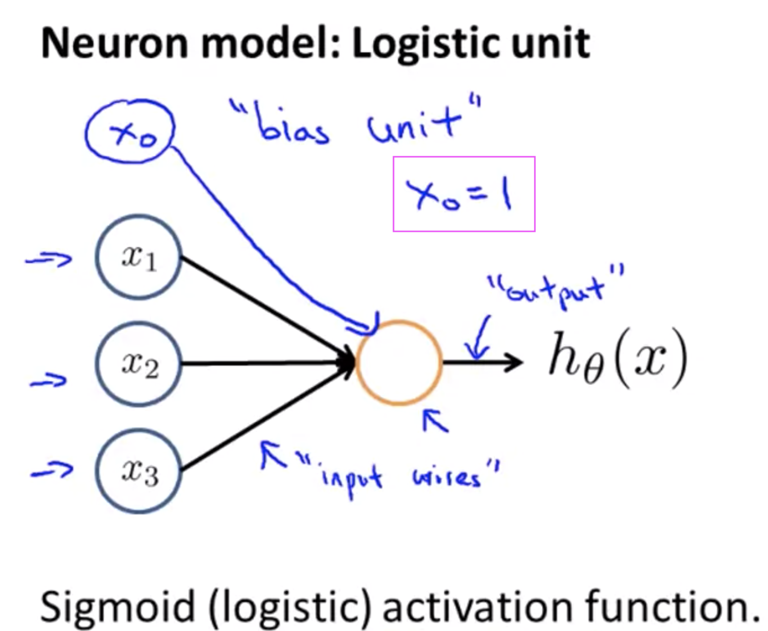
Neural Network:

An input layer, an output layer, and hidden layer(s).

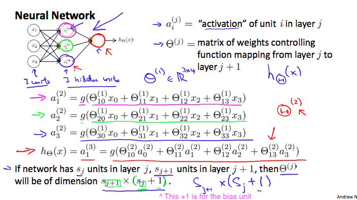
Why Hidden Layers?

With the help of the hidden layer, we can learn some pretty interesting and complex features and therefore we can end up with a better hypothesis than if we were constrained to use the raw features $x_1, x_2, x_3$ or if you will constrain to say choose the polynomial terms of $x_1, x_2, x_3$. But instead, this algorithm has the flexibility to try to learn whatever features at once, using these $a_1, a_2, a_3$ in order to feed into this last unit that’s essentially a logistic regression here.

The neural network can use this hidden there to compute more complex features to feed into this final output layer and it can learn more complex hypotheses.

Applications

And and Or can be computed using two layers: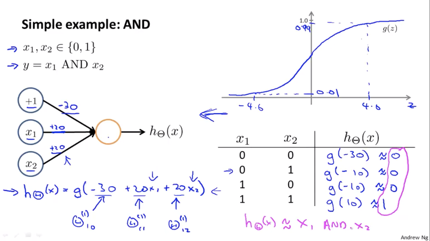

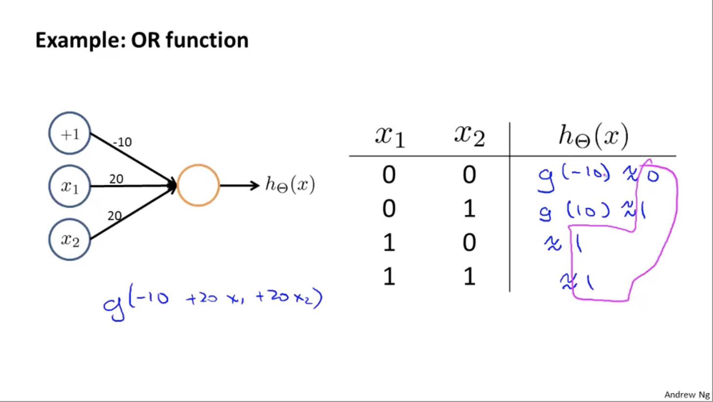
If we group up some neural networks we have, we can implement XNOR: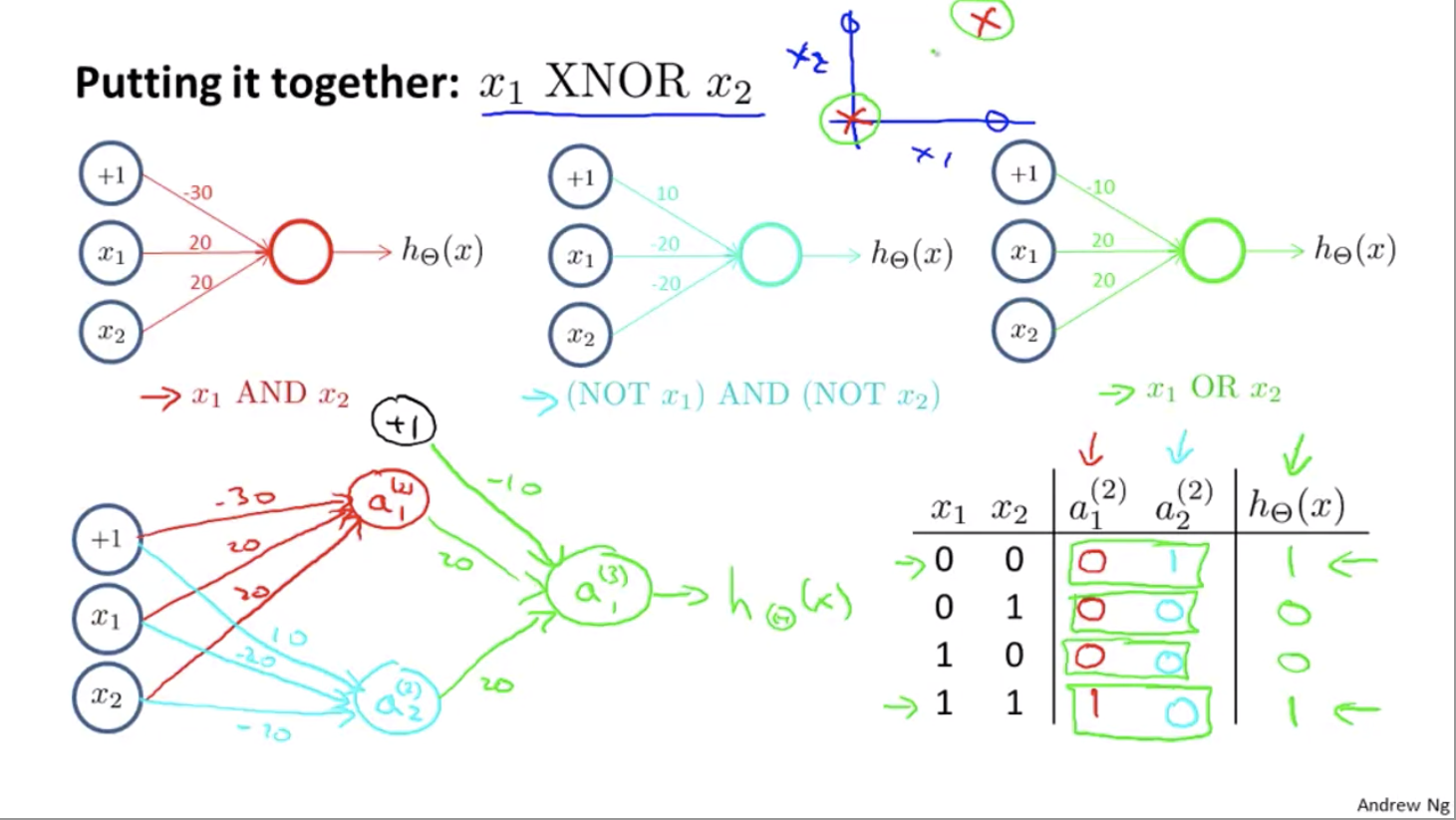

That’s why neural networks can compute pretty complicated functions. When we have multiple layers, we have a relatively simple function of the inputs of the second layer. But the third layer can build on that to complete even more complex functions, and then the layer after that can compute even more complex functions.

Multiclass Classification

Let’s say that we have a computer vision example, where we’re trying to recognize four categories of objects, and given an image we want to decide if it is a pedestrian, a car, a motorcycle, or a truck.

If that’s the case, what we would do is we would build a neural network with four output units so that our neural network now outputs a vector of four numbers. Then (ideally) $[1, 0, 0, 0]$ will represent a pedestrian, $[0, 1, 0, 0]$ will represent a car, etc.

Week 5 - Neural Networks: Learning

Cost Function

Recall that the regularized cost function of logistic regression is

$$J(\theta) = -\frac{1}{m}\sum_{i=1}^{m}y^{(i)}\log(h_\theta(x^{(i)})) + (1-y^{(i)})\log(1-h_\theta(x^{(i)})) + \frac{\lambda}{2m}\sum_{j=1}^{m}\theta_j^2$$

Note that the second summation is from 1 to n, as we don’t regularize the biased term $\theta_0$.

The cost function of the neural network is:

$$h_\Theta(x) \in R^K \;\;\; (h_\Theta(x))_i = i^{th} \text{output} \\ J(\Theta) = -\frac{1}{m}\sum_{i=1}^{m}\sum_{k=1}^{K}y_k^{(i)}\log(h_\Theta(x^{(i)}))_k + (1-y_k^{(i)})\log(1-(h_\Theta(x^{(i)}))_k) + \frac{\lambda}{2m}\sum_{l=1}^{L-1}\sum_{i=1}^{s_l}\sum_{j=1}^{s_l+1}(\Theta_{ji}^{(l)})^2$$

For the regularization term:
The number of columns in our current theta matrix is equal to the number of nodes in our current layer (including the bias unit). The number of rows in our current theta matrix is equal to the number of nodes in the next layer (excluding the bias unit). As before with logistic regression, we square every term.

Backpropagation Algorithm

• Goal: find the $\Theta$ that minimizes $J(\Theta)$.
  i.e. find $\min_{\Theta} J(\Theta)$
• Intuition: $\delta_j^{(l)}$ is the “error” of node $j$ in layer $l$

e.g. if $l = 4$ (we have 4 layers), then

$$\delta^{(4)} = a^{(4)} - y \\ \delta^{(3)} = (\Theta^{(3)})^T\delta^{(4)} .*g'(z^{(3)}) \;\;\;\text{ where .* is element-wise product}\\ \delta^{(2)} = (\Theta^{(2)})^T\delta^{(3)} .*g'(z^{(2)}) \\ \text{No } \delta^{(1)} \text{ since that is the feature we have and it has no errors}$$

Note that when we take the derivative of $g$, we can get $g’(z^{(3)}) = a^{(3)} .* (1 - a^{(3)})$

As for the partial derivative: if we ignore the regularization, then $\frac{\partial{}}{\partial{\Theta_{ij}^{(l)}}}J(\Theta) = a_j^{(l)}d_i^{(l+1)}$

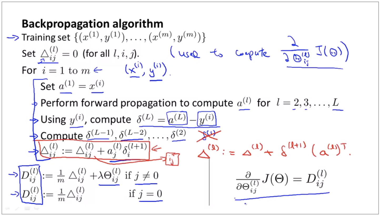
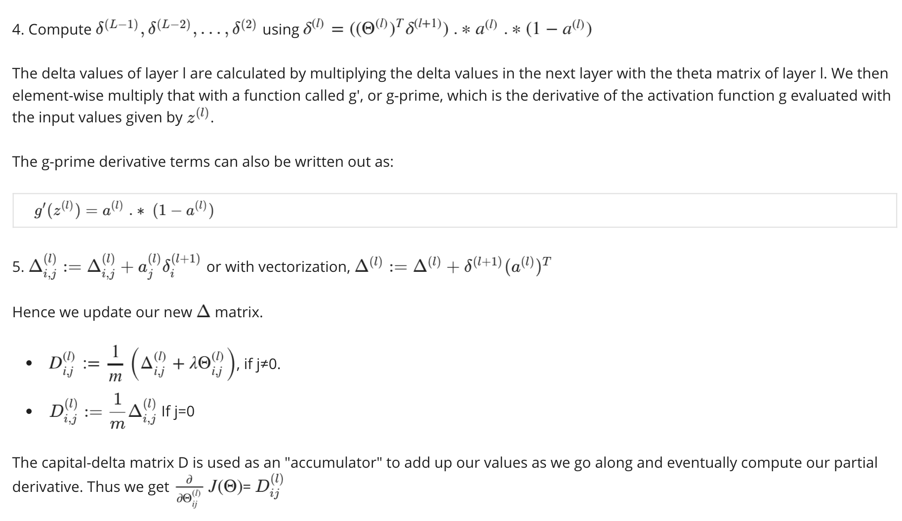
Steps in detail: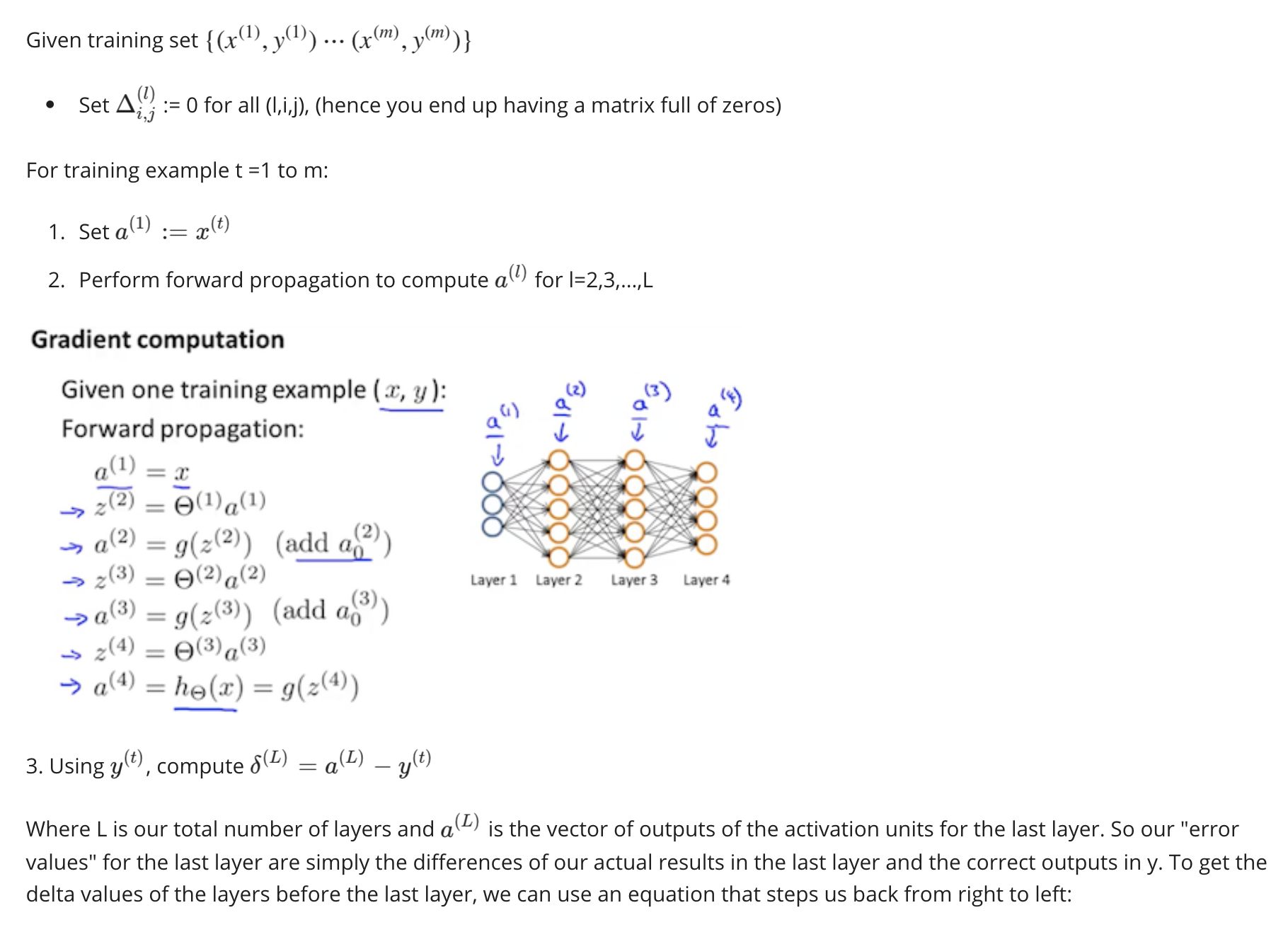

Implementation Note: Unrolling Parameters: Matrix -> Vector

The advantages of the matrix representation:

• more convenient when doing forward propagation and backpropagation
• easier for vectorized implementations

The advantage of the vector representation:

• when using the advanced optimization algorithms, those algorithms tend to assume that we have all of our parameters unrolled into a big long vector

Gradient Checking

$$\frac{\partial{}}{\partial{\Theta}} J(\Theta) \approx \frac{J(\Theta + \epsilon) - J(\Theta - \epsilon)}{2\epsilon}$$

where $\epsilon$ is a very small number.

For a parameter vector $\theta$, the gradient checking applies as follows: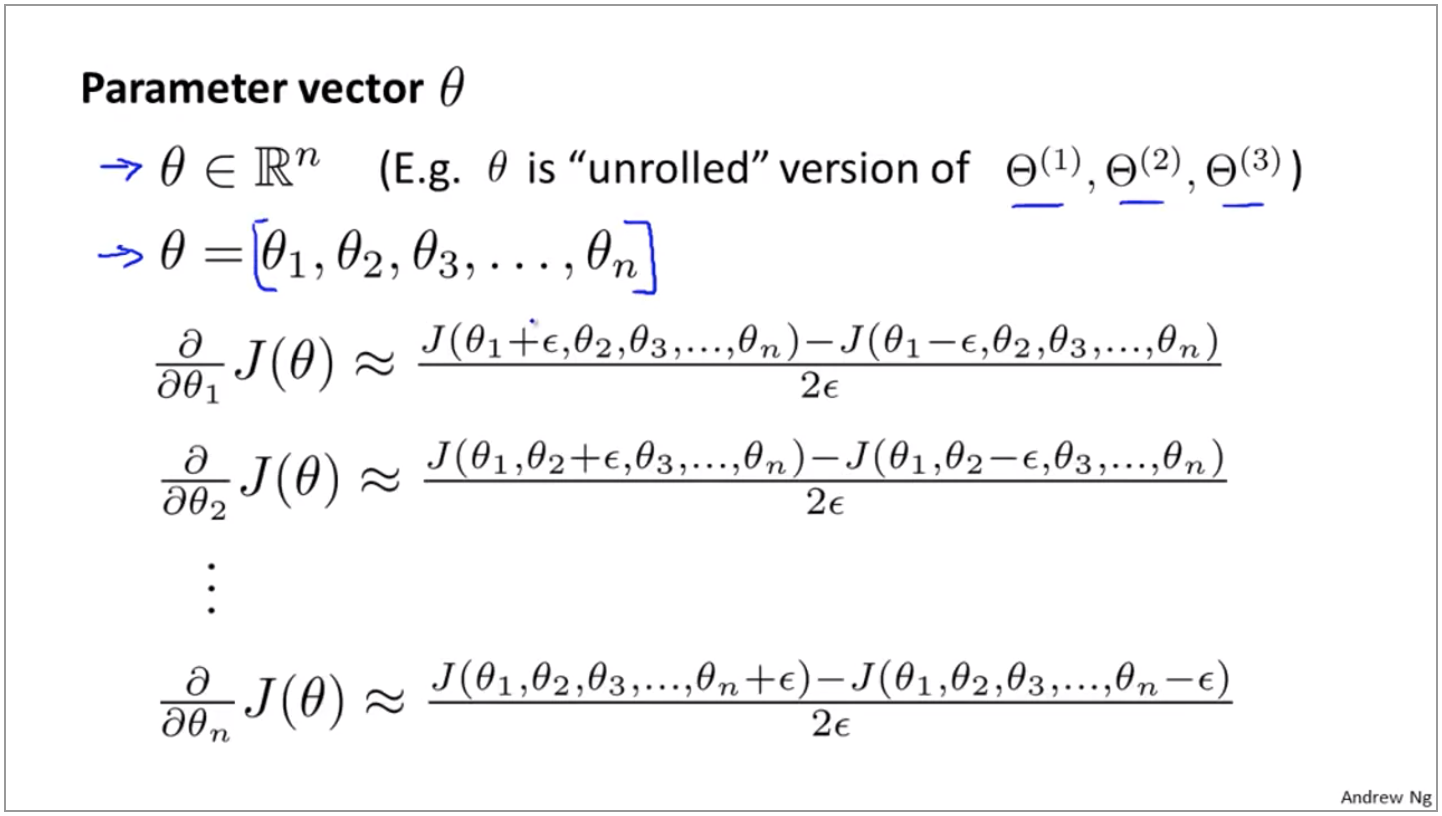

How gradient checking works:

1. First, run backpropagation to get DVec
2. Then, run the numerical gradient algorithm as described above to get gradApprox
3. Check that gradApprox is approximately the same as DVec.
4. Turn off the numerical gradient algorithm, since it is very slow (compared to backpropagation).
5. Accept DVec as the result of backpropagation

Random Initialization

What should we set the init values of $\Theta$ to be?
First, consider all zero ($\Theta{ij}^{(l)} = 0 \;\; \forall i,j, l$). The problem of this is that for a certain $i$ in layer $l$, $\Theta{ij}^{(l)}$ will be the same for all $j$ (see the figure below: the blue arrows will have the same weight, the red arrows will have the same weight, and the green arrows will have the same weight).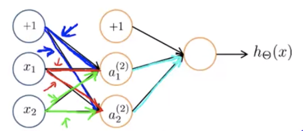

Generally speaking, the same will also happen no matter we set $\Theta_{ij}^{(l)} \;\; \forall i,j, l$ to be 0 or some other value — as long as all elements have the same value, it fails to break the symmetry.

The correct way to initialize the values is to set each elements $\Theta_{ij}^{(l)} \;\; \forall i,j, l$ to be a random value in $[-\epsilon, \epsilon]$

Wrap Up

Setting up a neural network:

• Number of input units: the dimension of features $x^{(i)}$
• Number of output units: number of classes
• Reasonable default: 1 hidden layer, or if > 1 hidden layer, then each hidden layer has the same number of hidden units

Training a neural network:

1. Randomly initialize weights
2. Implement forward propagation to get $h_\Theta(x^{(i)})$ for any $x^{(i)}$.
3. Implement code to comput cost function$J(\Theta)$
4. Implement back parpagation to compute partial derivatives $\frac{\partial}{\partial\Theta_{jk}^{(l)}}J(\Theta)$
5. Use gradient checking to compare $\frac{\partial}{\partial\Theta_{jk}^{(l)}}J(\Theta)$ computed using backpropagation v.s. using numerical estimmate of gradient of $J(\Theta)$.
   Then disable gradient checking, since it’s very slow.
6. Use gradient descent or advanced optimization method with backpropagation to try to minimize $J(\Theta)$ as a function of parameters $\Theta$

The cost function for the neural network is not convex, i.e. we may end up in a local optimum rather than a global optimum. But in most cases, this is not a big deal, because the algorithm will usually find a good enough local optimum.

Week 6 - Advice for Applying Machine Learning, Machine Learning System Design

Debugging a Learning Algorithm

If there are errors in the prediction, what should we do?

• Get more training examples
• Try smaller set of features
• Try getting additional features
• Try adding polynomial features ($x_1^2, x_2^2, x_1x_2$ etc)
• Try decreasing $\lambda$
• Try increasing $\lambda$

The Test Set Error

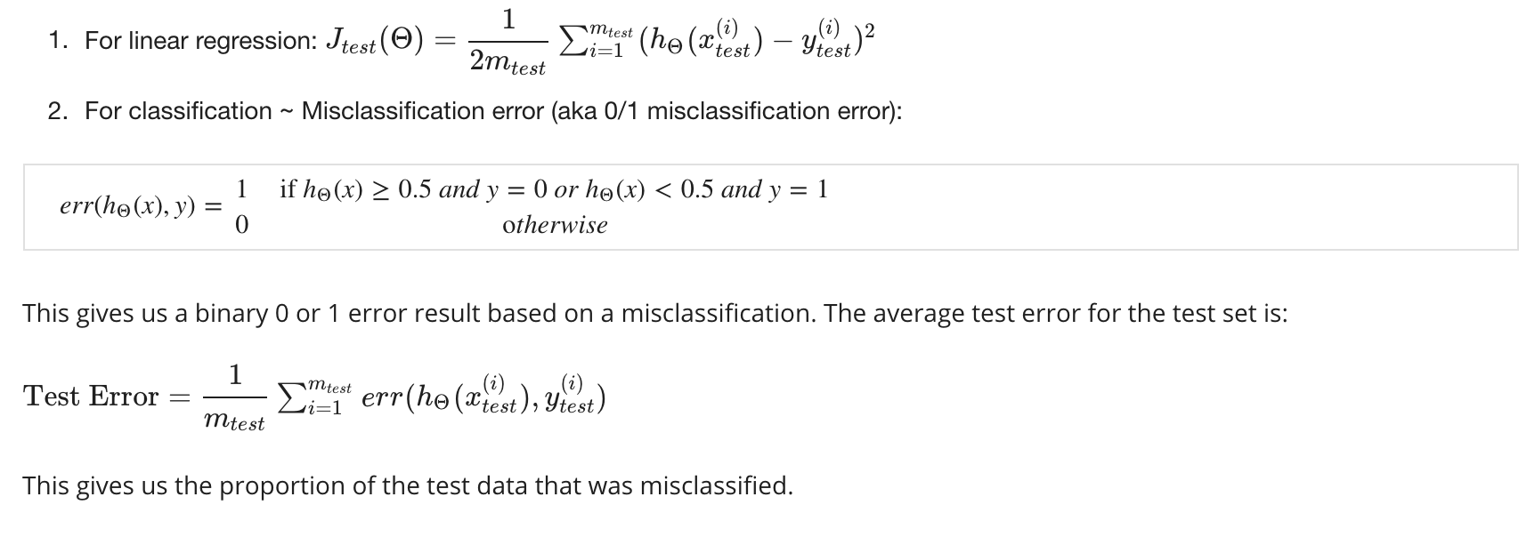
Previously, we divide our set into 70% training set and 30% testing set.

But this has a problem — when we try to find the degree of the polynomial that fits the data, we try from d = 1 to, say, d = 10. We then calculate $J_{test}(\Theta)$ for each different degree, and find the degree d that minimizes the cost.

This is usually an overly optimistic estimate because we choose the model for the test set based on the same test set’s performance.

In order to address this problem, let’s divide the data in this way: 60% training set, 20% cross-validation (CV) set, and 20% test set.

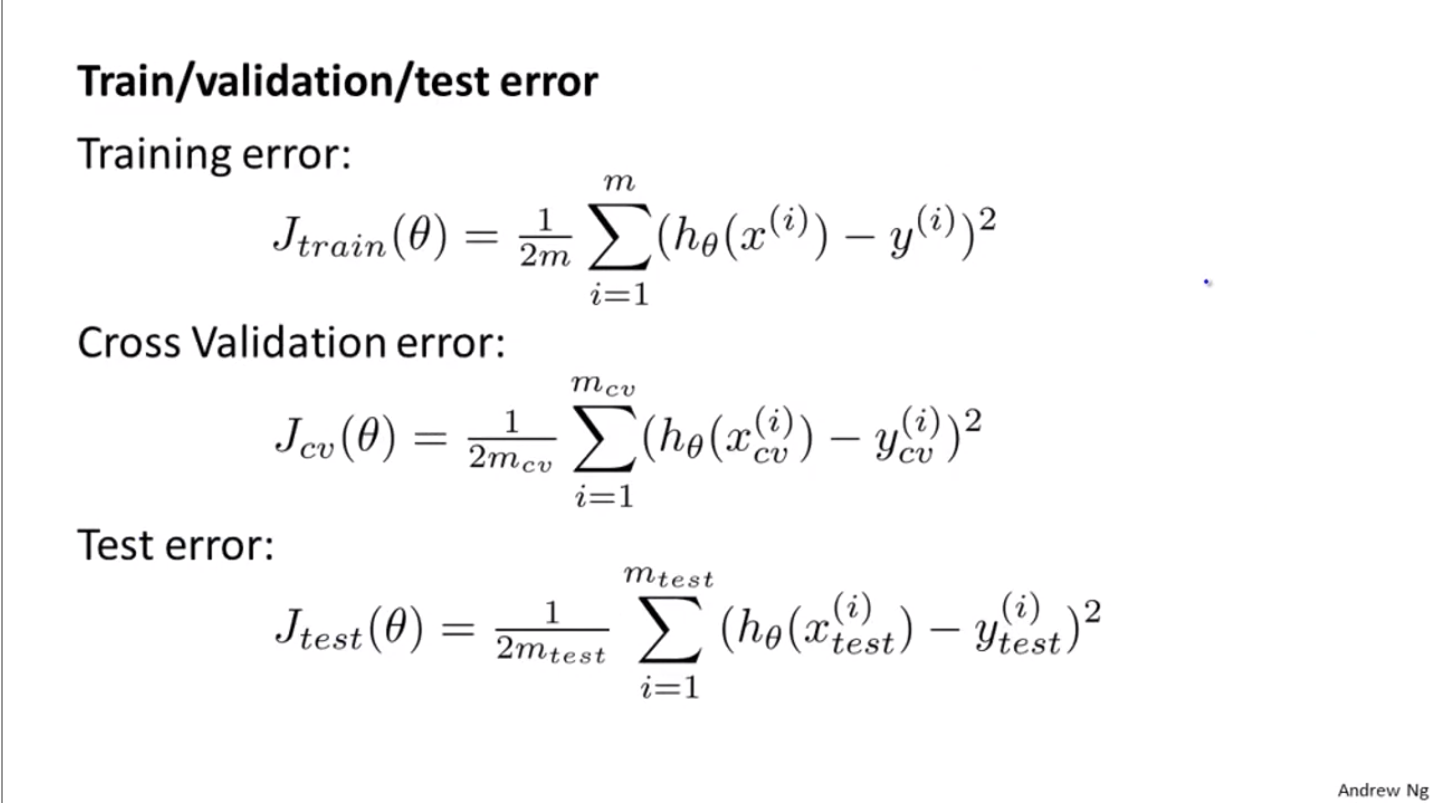
So back to the problem to find the best degree d: instead of using the test set to select the degree, we use the cross-validation set to find the d and estimate the error on the test set.

Bias vs Variance

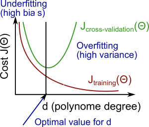
x	High bias (underfit)	High variance (overfit)
$J_{train}(\Theta)$	high	low
$J_{cv}(\Theta)$	high (approx. the same as $J_{train}(\Theta)$)	high ($J{cv}(\Theta) >> J{train}(\Theta)$)

Choosing the Regularization Parameter $\lambda$

Similarly, when we choose the regularization parameter $\lambda$ for a fixed-degreed model, we can also use the training/cv/test method as above. We would try $\lambda = 0, 0.01, 0.02, 0.04, 0.08, \ldots, 10.24$ and find the $\Theta$ that minimized $J_{cv}(\Theta)$ and use that model on our test set.

Learning Curves

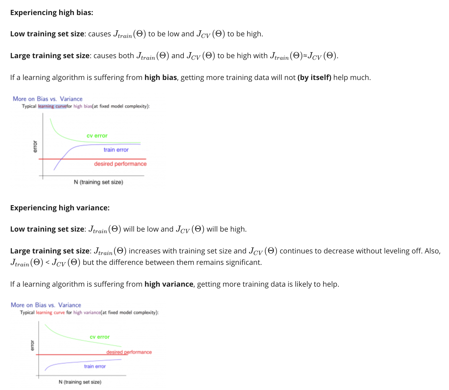
Deciding What to Do

Back to the examples we discussed at the beginning of this week:

• Get more training examples —> fixes high variance
• Try smaller set of features —> fixes high variance
• Try getting additional features —> fixes high bias
• Try adding polynomial features ($x_1^2, x_2^2, x_1x_2$ etc) —> fixes high bias
• Try decreasing $\lambda$ —> fixes high bias
• Try increasing $\lambda$ —> fixes high variance

Neural Network and Underfitting/Overfitting

• Small neural networks = fewer parameters = more prone to underfitting
• Large neural networks = more parameters = more prone to overfitting
• The number of hidden layers: using a single hidden layer is a reasonable default, but we can also try to find a training cross-validation and try training neural networks with one hidden layer or more hidden layers, and see which of those neural networks performs best on the cross-validation sets.

Machine Learning System Design

Instead of using gut feeling and starting with a carefully-designed algorithm, try to start with something quick and dirty and test it on cross-validation data quickly.

Plot learning curves and figure out how to improve our algorithm.

It’s usually a better practice to let the error tell us where to spend time for improvement, rather than spending much time on design.

Once the errors are found, manually go through the errors and find specifically a way to improve. (e.g. when building a quick and dirty algorithm for email spam classifier, we found that many “password-stealing” emails are not classified as spams. In this case, we can focus on how to improve the performance of our algorithm on detecting this kind of emails)

Skewed Classes

We have a lot more examples from one class than from the other class. (e.g. 99.5% cancers are benign, 0.5% cancers are malignant)

If we have very skewed classes, it becomes much harder to use just classification accuracy, because we can get very high classification accuracies or very low errors, and it’s not always clear if doing so is really improving the quality of your classifier. (e.g. predicting all cancers to be benign gives us 0.5% error, but it doesn’t seem like a good classifier)

Precision and Recall

Precision = # of true positives / # of all predicted positives
Recall = # of true positives / # of all actual positives

High precision & high recall means that the algorithm is doing well even on skewed classes.

Cancer example:
Logistic regression:

$$\text{Predict} = \begin{cases} 1 \text{ if } y \geq a \\ 0 \text{ if } y < a\\ \end{cases}$$

• Suppose we want to predict y=1 (cancer) only when very confident: increase $a$ - high precision, low recall
• Suppose we want to avoid missing too many cases of cancer: decrease $a$ - high recall, low precision.

Say we have multiple algorithms that have different precisions and recalls. Which one is the best of them?

Let’s use “F score”: $\frac{2PR}{P+R}$.

High F score = better algorithm.

F score equals 0 if P=0 and R=0. F score equals 1 if P=1 and R=1.

Week 7 - Support Vector Machines

Large Margin Classification

Support vector machines:

Recall that the regularized cost function of logistic regression is

$$J(\theta) = \frac{1}{m}[\sum_{i=1}^{m}y^{(i)}(-\log(h_\theta(x^{(i)}))) + (1-y^{(i)})(-\log(1-h_\theta(x^{(i)})))] + \frac{\lambda}{2m}\sum_{j=1}^{m}\theta_j^2$$

and we want to find the $\theta$ such that

$$\min_{\theta} \frac{1}{m}[\sum_{i=1}^{m}y^{(i)}(-\log(h_\theta(x^{(i)}))) + (1-y^{(i)})(-\log(1-h_\theta(x^{(i)})))] + \frac{\lambda}{2m}\sum_{j=1}^{m}\theta_j^2$$

Note that $m$ is a constant in this formula. The value of $m$ doesn’t affect $\theta$.

Let $A = \sum{i=1}^{m}y^{(i)}(-\log(h\theta(x^{(i)}))) + (1-y^{(i)})(-\log(1-h\theta(x^{(i)})))$ and $B=\frac{1}{2}\sum{j=1}^{m}\theta_j^2$. Instead of writing $A+\lambda B$, let’s rewrite it as $CA+B$ (we can see $C$ as $\frac{1}{\lambda}$)

So our formula is:

$$\min_{\theta} C[\sum_{i=1}^{m}y^{(i)}(-\log(h_\theta(x^{(i)}))) + (1-y^{(i)})(-\log(1-h_\theta(x^{(i)})))] + \frac{1}{2}\sum_{j=1}^{m}\theta_j^2$$

Support Vector Machine

We want $\sum{i=1}^{m}y^{(i)}(-\log(h\theta(x^{(i)}))) + (1-y^{(i)})(-\log(1-h_\theta(x^{(i)})))$ to be as small as possible (close to 0), so we want to meet the requirements below:

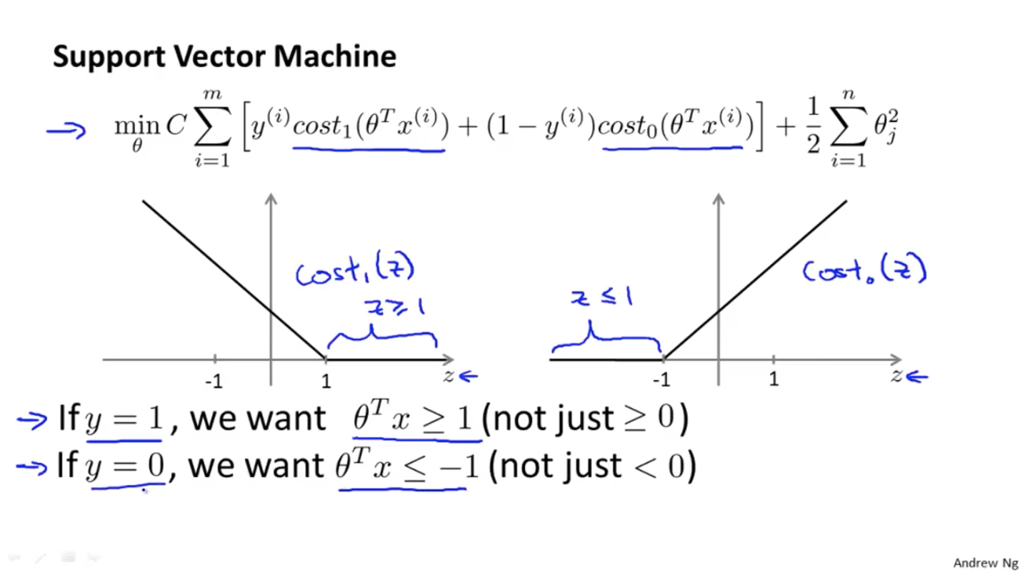
The algorithm will choose the black line as the boundary over the pink line and the green line, as the black line has a larger minimum distance between the positive and negative samples (see the blue bands on both sides of the black line)

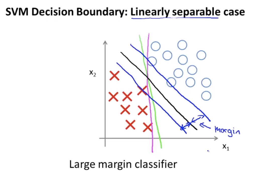
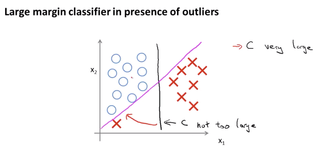
The value of $C$ decides how fast the boundary will change when there are outliers. For example, in the figure below, the boundary was the black line. If we add an outlier:

• if $C$ is very large, the new boundary given by the algorithm will be the pink line (but we might not want the boundary to be this sensitive on one outlier)
• if $C$ is not very large, the new boundary given by the algorithm will still stay around the black line

Kernels

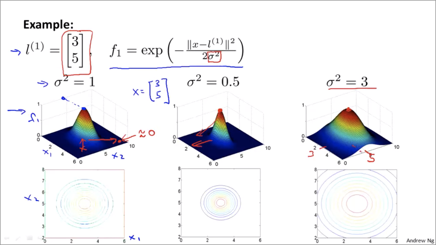
Let’s define $f_1 = \text{similarity}(x, l^{(1)}) = \exp (-\frac{||x - l^{(1)}||^2}{2 \sigma^2})$

What does similarity represent? It represents how close the point $x$ is to the feature we’re talking about (in this case $l^{(i)}$).

If the point $x$ is close to the feature point $l^{(i)}$, then the numerator ($||x - l^{(1)}||^2$) is small, so $f$ is close to 1.

If the point $x$ is far from the feature point $l^{(i)}$, then the numerator ($||x - l^{(1)}||^2$) is large, so $f$ is close to 0.

As for the $\sigma$ in the denominator, it controls how fast the similarity drops from 1 to 0 as the point moves further away from the feature.

Choosing Landmarks

How can we choose landmarks?
Let the landmarks to be at exactly the same locations as the training samples.

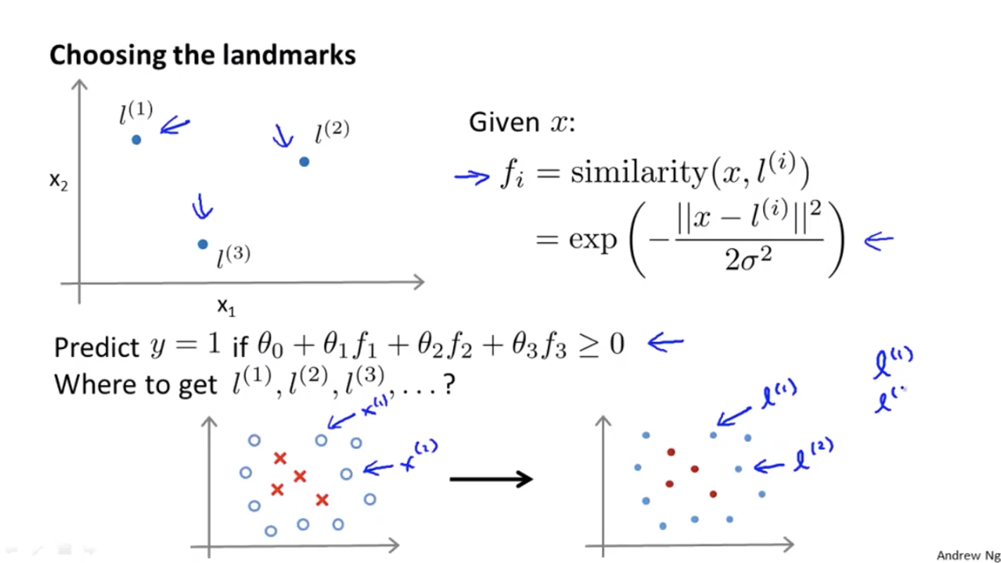
That is, given training samples $(x^{(1)}, y^{(1)}), (x^{(2)}, y^{(2)}), \ldots, (x^{(m)}, y^{(m)})$, let $l^{(1)} = x^{(1)}, l^{(2)} = x^{(2)}, \ldots, l^{(m)} = x^{(m)}$.

For training sample $(x^{(i)}, y^{(i)})$, we map $x^{(i)}$ to

$$f = \begin{bmatrix} f_1^{(i)}\\ f_2^{(i)}\\ \ldots\\ f_m^{(i)} \end{bmatrix}$$

where

$$f_1^{(i)} = \text{sim}(x^{(i)}, l^{(1)}), \\ \ldots, \\ f_i^{(i)} = \text{sim}(x^{(i)}, l^{(i)}) = \text{sim}(x^{(i)}, x^{(i)}) = 1, \\ \ldots, \\ f_m^{(i)} = \text{sim}(x^{(i)}, l^{(m)})$$

SVM with Kernels

We pad $f_0^{(i)} = 1$ to the vector $f$ we have above and get a $m+1$-dimention vector.
To train the algorithm:

$$\min_{\theta} C[\sum_{i=1}^{m}y^{(i)}\text{cost1}(\theta^Tf^{(i)}) + (1-y^{(i)})\text{cost0}(\theta^Tf^{(i)})] + \frac{1}{2}\sum_{j=1}^{m}\theta_j^2$$

See the figure above for the definition of cost0 and cost1.

SVM Parameters

$C(=\frac{1}{\lambda})$:

• Large C: lower bias, high variance
• Small C: higher bias, low variance

$\sigma$:

• Large $\sigma$: feature varies more smoothly. Higher bias, lower variance.
• Small $\sigma$: feature varies less smoothly. Lower bias, higher variance.

Note:

Do perform feature scaling before using Gaussian Kernel.

If not scaled, e.g. feature 1 is the size of the house (~1000 sqft), and feature 2 is the number of bedrooms (1-5), then the distance $||x-l||^2 = (x_1-l_1)^2+(x_2-l_2)^2+\ldots$ will be dominated by the first feature.

Logistic Regression v.s. SVM: when to use which?

Let n be the number of features, and m be the number of training samples.

• If n is large (relative to m), use logistic regression, or SVM without a kernel (linear kernel), because we have so many features but a small training set, so a linear function will probably do fine
• If n is small and m is intermediate, use SVM with Gaussian kernel
• If n is small but m is large, then add more features and use logistic regression, or SVM without a kernel (linear kernel), because SVM with Gaussian will be slow if we have too many training samples

Week 8 - Unsupervised Learning, Dimensionality Reduction

Unsupervised Learning

Supervised learning:
given a labeled training set and the goal is to find the decision boundary that separates the positive label examples and the negative label examples.

Unsupervised learning:
given data that does not have any labels associated with it and we just ask the algorithm find some structure in the data for us.

Examples of structures: clusters (clustering algorithm)

K-Means Algorithm: a Clustering Algorithm

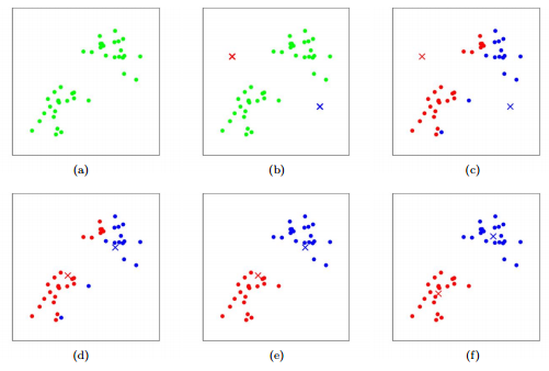
a. List all training examples.
b. Init: randomly find two cluster centroids (red and blue)
c. Cluster assignment: loop through all training examples. For each of them, assign it to the red centroid if it’s closer to the red centroid, or assign it to the blue centroid if it’s closer to the blue centroid.
d. Move centroid: calculate the mean of the red training examples, and move the red centroid to there. Same for blue centroid.
e. Repeat step 2 and 3 — new round of color assignment, move centroids, etc.
f. After a few rounds, the cluster centroid will not change during the move centroid step.

For the move centroid step: what if no points are assigned to this centroid?
In this case, let’s just eliminate the centroid, and our goal will change from “assign the points to K clusters” to “assign the points to K-1 clusters”

If the clusters are non-separated, the K-Means algorithm will still try to cluster them into K clusters.

Optimization Objective

The supervised learning algorithms we’ve seen like linear regression and logistic regression have an optimization objective or some cost function that the algorithm was trying to minimize.

It turns out that K-Means also has an optimization objective or a cost function that it’s trying to minimize.

Notations:

• $c^{(i)}$: index of cluster $(1, 2, \ldots, K)$ to which example $x^{(i)}$ is currently assigned
• $\mu_k$: cluster centroid $k$
• $\mu_{c^{(i)}}$: cluster centroid of cluster to which example $x^{(i)}$ has been assigned

e.g. $x^{(i)}$ is assigned to cluster 5, then $c^{(i)} = 5$, $\mu_{c^{(i)}} = \mu_5$

The cost function (aka distortion) is:

$$J(c^{(1)}, \ldots, c^{(m)}, \mu _1, \ldots, \mu _K) = \frac{1}{m} \sum_{i=1}^m ||x^{(i)} - \mu _{c^{(i)}}||^2$$

Note that $||x^{(i)} - \mu_{c^{(i)}}||^2$ is the distance between the training example and the cluster centroid it’s assigned to.

And the goal is:

$$\min_{c^{(1)}, \ldots, c^{(m)}, \mu_1, \ldots, \mu_K} J(c^{(1)}, \ldots, c^{(m)}, \mu_1, \ldots, \mu_K)$$

Note that it’s not possible for the cost function to increase during each iteration. If you see your cost increasing, there must be something wrong with your code.

Random Initialization of Clusters

Randomly pick K training examples and set them to be $\mu_1, \ldots, \mu_k$.

If you don’t want to stuck at a local optimum, do multiple retries. For example, do 100 different random initializations and find the best clustering (lowest cost).

If K is small, say less than 10, then multiple random initializations is very helpful to find a good clustering. But if K is large, say 100, then having multiple random initializations is less likely to make a huge difference.

That’s because when K is large, our first random initialization will probably give us a decent solution. All retries after that will provide similar results.

Choosing the Number of Clusters

1. Elbow method (could work, but not usually doing well)
   

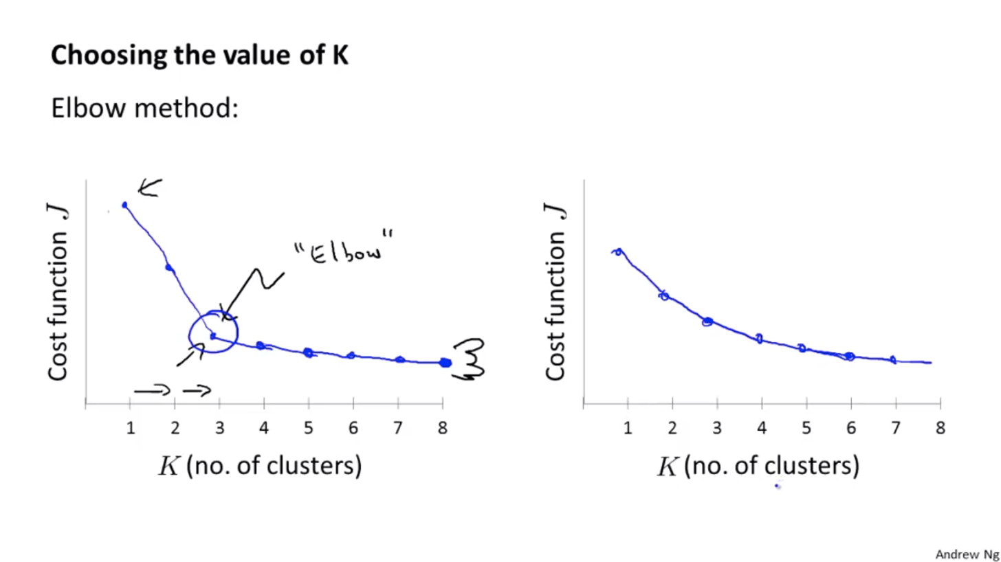
But sometimes it’s hard to find the elbow, see the picture on the RHS.

1. Think about the later purpose. How many clusters do we want?
   e.g. T-shirt size, do we want 3 sizes (S, M, L) or 5 sizes (XS, S, M, L, XL)?

Data Compression

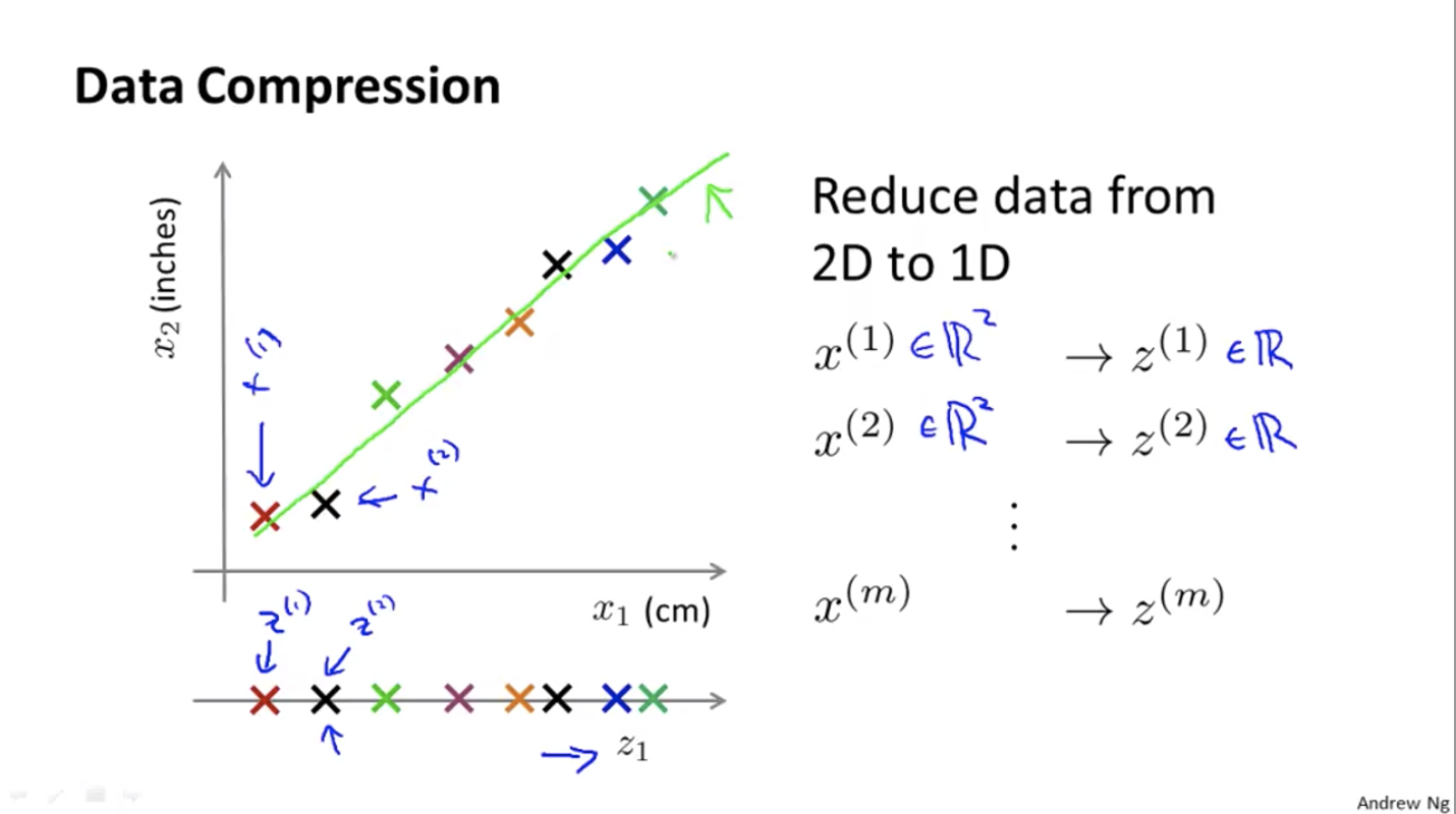
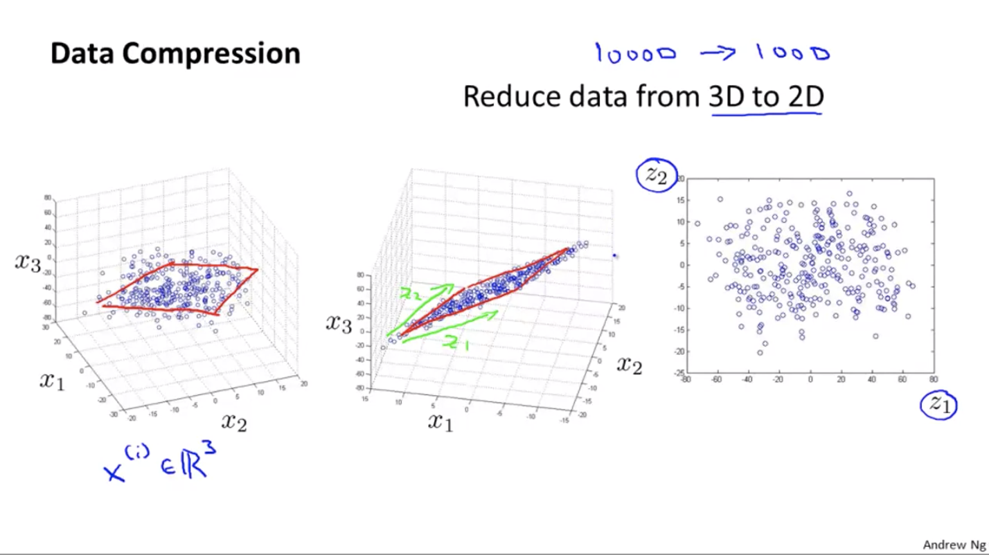
Basic idea: project the points in a N-dimension space to a (N-1)-dimension space.

Principal Components Analysis

For the problem of dimensionality reduction, the most commonly used algorithm is principal components analysis, or PCA.

The goal of PCA:

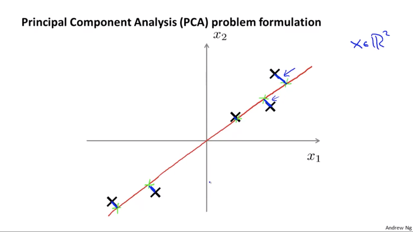
The length of those blue line segments is called the projection error. What PCA does is to find a lower-dimensional surface onto which to project the data in order to minimize the error.
Note that PCA is different from linear regression (least square). For linear regression, the blue line segments are always vertical, while for PCA, the blue line segments are perpendicular to the red line.

PCA Algorithm — reduce n-dimensional vectors to k-dimensional

1. Compute “covariance matrix” $$\Sigma = \frac{1}{m} \sum_{i=1}^n(x^{(i)})(x^{(i)})^T$$
2. Computer eigenvectors of matrix $\Sigma$ $$[U, S, V] = svd(sigma) // singular value decomposition$$
3. What we need from above is the $U$ matrix. Suppose $(x^{(i)})$ is $n \times 1$, then $U$ is a $n \times n$ matrix, and each column of it will be the $u^{(i)}$ vector we want (n vectors in total). To get a k-dimensional space, we can just take the first $k$ columns. Let’s call it $U_{reduce}$ of shape $n \times k$.
4. Then, for each $x \in R^n$, we want to find a $z \in R^k$ which is a lower-dimensional representation of our vector. Then $z = U_{reduce}^T * x$.

Reconstruction from the Compressed Representation

The above algorithm shows how to reduce an n-dimensional vector to a k-dimensional vector. How can we do it backward?

$$x_{approx}^{(i)} = U_{reduce} * z^{(i)}$$

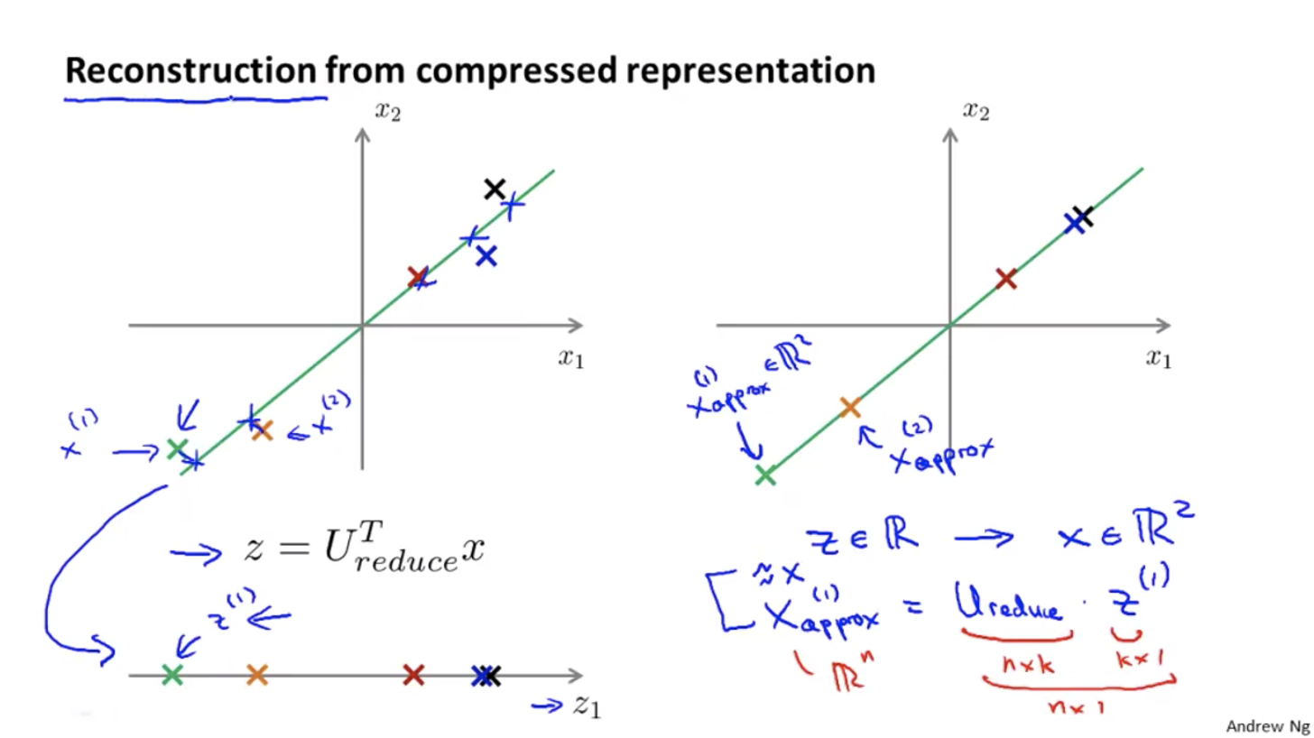
How to Choose k for PCA

We want to choose a $k$ such that “99% variance is retained”

$$\frac{\text{average squared projection error}}{\text{total variation}} = \frac{\frac{1}{m}\sum_{i=1}^m||x^{(i)} - x^{(i)}_{approx}||^2}{\frac{1}{m}\sum_{i=1}^m||x^{(i)} ||^2} \leq 0.01$$

In real life, in order to retain 99% of the variance, we can often reduce the dimension of the data significantly and still retain most of the variance.

That’s because, for most real-life data, many features are highly correlated, so it turns out to be possible to compress the data a lot and still retain 99% of the variance.

The algorithm is simply starting from $k = 1$ and check if the result is less than 0.01. If it works, then take the value, else increment $k$ by 1 and repeat.

However, it’s very inefficient.

Instead, let’s use the $S$ in $[U, S, V] = svd(sigma)$.

$$S = \begin{bmatrix} S_{11} & 0 & \ldots & 0\\ 0 & S_{22} & \ldots & 0\\ 0 & 0 & \ddots & \vdots\\ 0 & \ldots & 0 & S_{nn} \end{bmatrix}$$

With this, the value above can be easily computed as

$$\frac{\frac{1}{m}\sum_{i=1}^m||x^{(i)} - x^{(i)}_{approx}||^2}{\frac{1}{m}\sum_{i=1}^m||x^{(i)} ||^2} = 1 - \frac{\sum_{i=1}^k S_{ii}}{\sum_{i=1}^n S_{ii}}$$

So we want

$$\frac{\sum_{i=1}^k S_{ii}}{\sum_{i=1}^n S_{ii}} \geq 0.99$$

Applying PCA

What PCA does is that it provides a mapping that reduces, say, $x^{(i)} \in R^{10000}$ to $z^{(i)} \in R^{1000}$. The mapping is defined by running PCA only on the training set, not the cross-validation set or the testing set.

So the training set will change from $(x^{(i)}, y^{(i)})$ to $(z^{(i)}, y^{(i)}) \;\; \forall i = 1, \ldots, m$. It will speed up our training.

But don’t abuse PCA. Don’t use PCA right away. Always try to train $(x^{(i)}, y^{(i)})$ first — only if it doesn’t work (e.g. very slow, very memory-consuming), then try to use PCA to do the mapping and train $(z^{(i)}, y^{(i)})$.

Week 9 - Anomaly Detection, Recommender Systems

Anomaly Detection

Given a set of points and a new point $x_{test}$, is it a normal case or an anomaly?

Gaussian (Normal) Distribution

$$x \thicksim N(\mu, \sigma^2)$$

where $\mu$ is the mean and $\sigma^2$ is the variance.

$$P(x; \mu, \sigma^2) = \frac{1}{\sigma \sqrt{2\pi}}\text{exp}(-\frac{(x-\mu)^2}{2\sigma^2})$$

When given a data set of $m$ points, how can we estimate a Gaussian distribution for them?

Let $\mu = \frac{1}{m} \sum{i=1}^m x^{(i)}$ and $\sigma^2 = \frac{1}{m} \sum{i=1}^m (x^{(i)} - \mu)^2$

Density Estimation

Let’s assume each feature is distributed according to Gaussian distribution.

That is, given the training set $x^{(1)}, x^{(2)}, \ldots, x^{(m)}$, each $x \in R^n$, we assume

$$x_1 \thicksim N(\mu_1, \sigma_1^2), \;x_2 \thicksim N(\mu_2, \sigma_2^2), \;\ldots, \;x_n \thicksim N(\mu_n, \sigma_n^2)$$

and that

$$P(x) = P(x_1; \mu_1, \sigma_1^2)P(x_2; \mu_2, \sigma_2^2) \ldots P(x_n; \mu_n, \sigma_n^2) \\ = \prod_{i=1}^n P(x_i; \mu_i, \sigma_i^2)$$

When given a new example $x$, calculate $P(x)$ as described above, and report anomaly if $P(x) < \epsilon$.

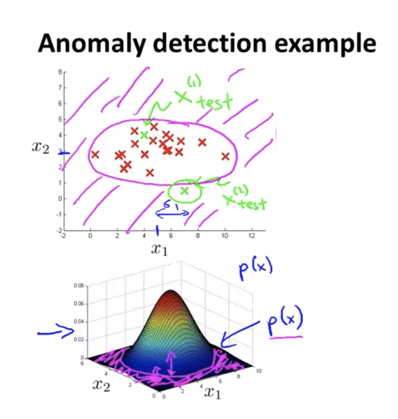
The pink shade on the figure on the top matches the pink shade on the figure on the bottom, which labels the area where $P(x) < \epsilon$.

Note that we usually use much more normal training samples than anomalous training samples (e.g. the engine example we use have 10000 normal engines and 20 flawed engines), so we might face a skewed class problem.

Anomaly Detection vs. Supervised Learning

Why do we use anomaly detection? Since we have a set of labeled data and we want to predict a new data’s label, why don’t we use supervised learning?

Anomaly Detection	Supervised Learning
A very small number of positive examples and a large number of negative examples	Large number of positive and negative examples
Many different types of anomalies, so it’s hard to “learn” what positive examples look like	Enough positive and negative examples for the algorithm to “get a sense of” what positive examples look like

Non-Gaussian Features

If some of the features don’t seem to be Gaussian, how can we transform it to be Gaussian?

One way is to use $P(\log(x_i); \mu_i, \sigma_i^2)$ rather than the usual $P(x_i; \mu_i, \sigma_i^2)$ form.

Some other examples are: $P(\log(x_i+1); \mu_i, \sigma_i^2)$, $P(\sqrt{x_i}; \mu_i, \sigma_i^2)$, $P(x_i^{0.75}; \mu_i, \sigma_i^2)$ etc. Just play around with it and make the data look more Gaussian.

Multivariate Gaussian Distribution

Sometimes, anomaly detection fails to recognize an anomaly, e.g. the green dot below. The algorithm has seen even less $x_1$ and even larger $x_2$, so it thinks the green dot is also normal.

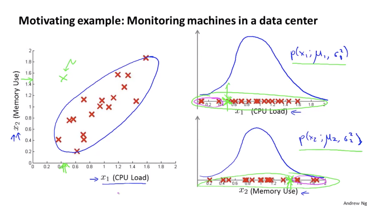
Multivariate Gaussian Distribution: Instead of modelling $P(x_1),P(x_2)$ separately, model $P(x)$ in one go — $P(x; \mu, \sigma)$.

Parameters: $\mu \in R^n, \; \Sigma \in R^{n \times n}$

Some examples:

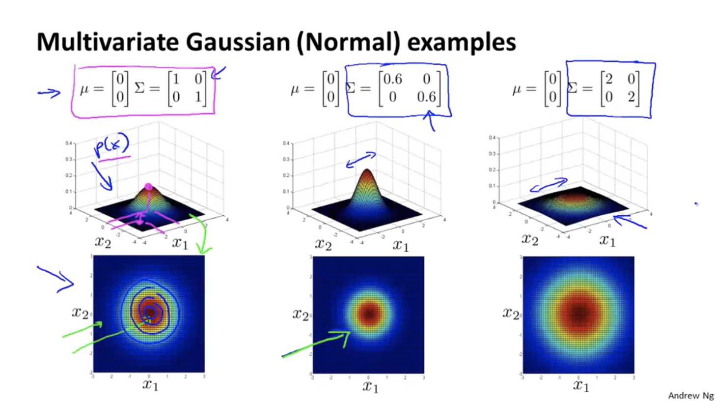
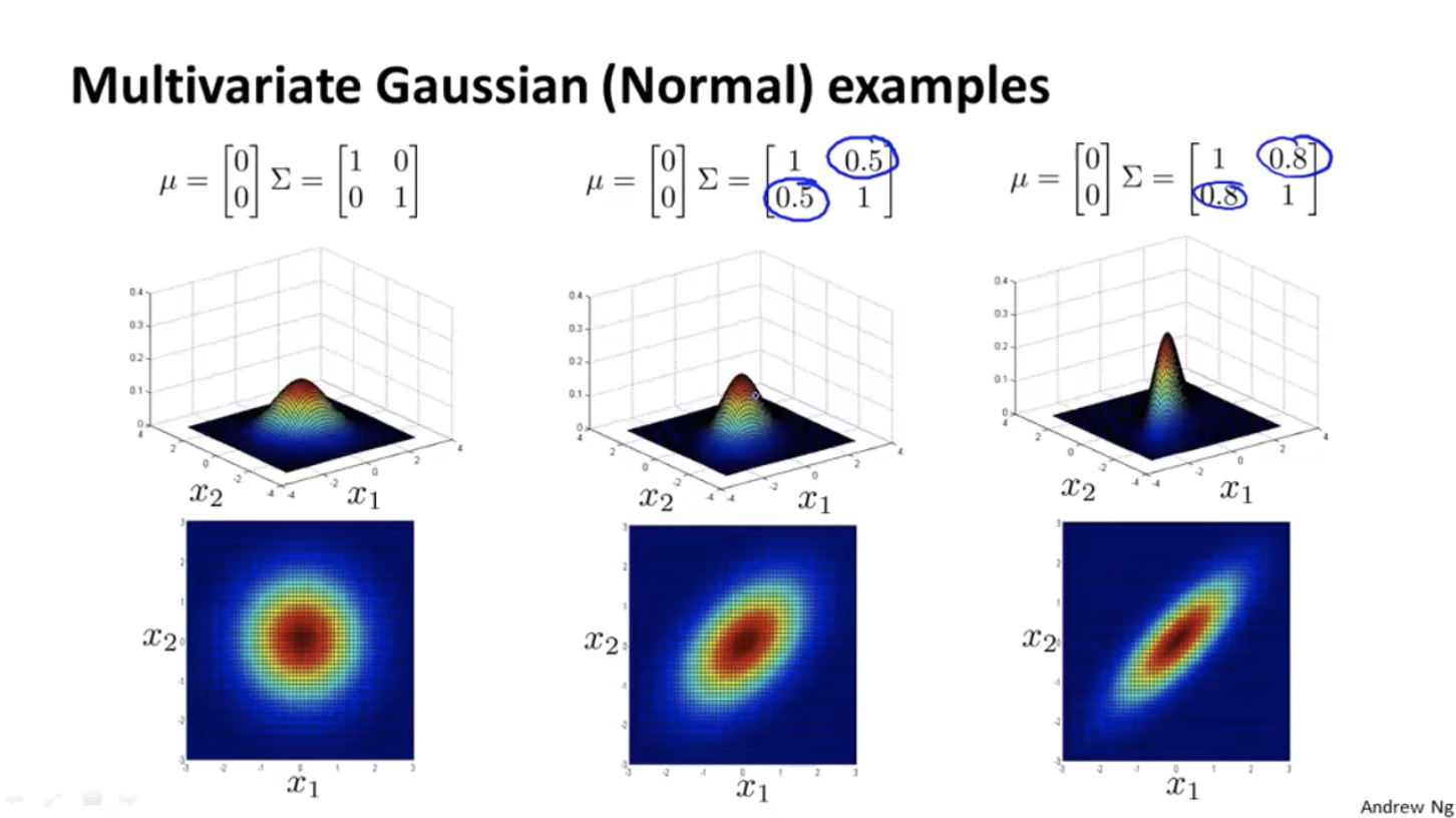
Multivariate Gaussian Distribution v.s. the Original Model

Turns out that for the original models, the contours of the graph are always axis aligned, i.e. their $\Sigma$ matrix’s non-diagonal entries are all 0, so the features’ covariance is 0.

With the original models, we can’t have contours that look like the 45 degrees tilted version as we have in the figure above.

The original version cannot capture the correlations between features, so sometimes we need to add some other features to make it work, e.g. apart from CPU_COUNT and NETWORK_SPEED, we may also need to add a feature CPU_COUNT^2 / NETWORK_SPEED.

Multivariate Gaussian Distribution, on the other hand, can capture the correlations between features automatically, so we don’t need to add new features.

But Multivariate Gaussian Distribution is computationally more expensive. So most of the time people use the original model plus manually design some new features.

Recommander Systems

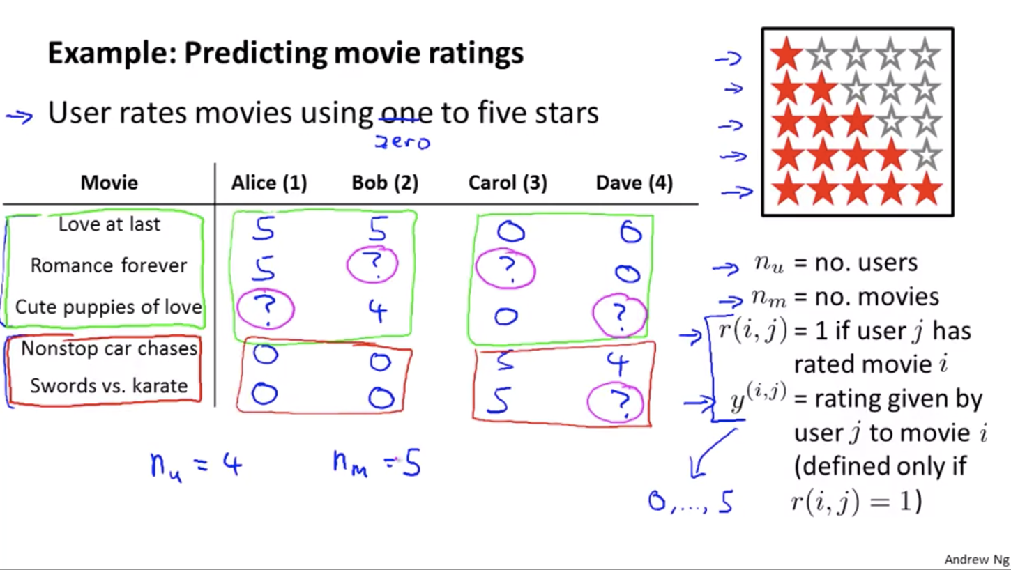
Content Based Recommendations

Optimization objective:

To learn $\theta^{(j)}$ (parameter for user j)

$$\min_{\theta^{(j)}} \frac{1}{2} \sum_{i:r(i, j) = 1} ((\theta^{(j)})^Tx^{(i)} - y^{(i, j)})^2 + \frac{\lambda}{2} \sum_{k = 1}^n(\theta_k^{(j)})^2$$

To learn $\theta^{(1)}, \theta^{(2)}, \ldots, \theta^{(n_u)}$ (parameter for all users):

$$\min_{\theta^{(1)}, \theta^{(2)}, \ldots, \theta^{(n_u)}} \frac{1}{2} \sum_{j=1}^{n_u} \sum_{i:r(i, j) = 1} ((\theta^{(j)})^Tx^{(i)} - y^{(i, j)})^2 + \frac{\lambda}{2} \sum_{j=1}^{n_u} \sum_{k = 1}^n(\theta_k^{(j)})^2$$

Note that originally the coefficients are $\frac{1}{2m^{(j)}}$ and $\frac{\lambda}{2m^{(j)}}$, but since $m^{(j)}$ is a constant, we can ignore it for both denumerator.

Gradient descent:

$$\theta_k^{(j)} := \theta_k^{(j)} - \alpha \sum_{i:r(i, j) = 1} ((\theta^{(j)})^Tx^{(i)} - y^{(i, j)}) x_k^{(i)} \;\; \text{when } k = 0 \\ \theta_k^{(j)} := \theta_k^{(j)} - \alpha \sum_{i:r(i, j) = 1} (((\theta^{(j)})^Tx^{(i)} - y^{(i, j)}) x_k^{(i)} + \lambda \theta_k^{(j)}) \;\; \text{when } k \neq 0$$

What if the movies are not content-based?

Collaborative Filtering

The algorithm has a very interesting property — feature learning. It means that the algorithm can start to learn for itself what features to use.

Let’s say we don’t know the features $x$ for the movies, but we do know the users’ ratings and their $\theta$’s.

From the four equations in the bottom right corner, we can roughly guess that $x^{(1)} = [1, 1.0, 0.0]^T$.

So the optimization algorithm will be given $\theta^{(1)}, \theta^{(2)}, \ldots, \theta^{(n_u)}$ to learn $x^{(i)}$:

$$\min_{x^{(i)}} \frac{1}{2} \sum_{j:r(i, j) = 1} ((\theta^{(j)})^Tx^{(i)} - y^{(i, j)})^2 + \frac{\lambda}{2} \sum_{k = 1}^n(\theta_k^{(i)})^2$$

Similarly, given $\theta^{(1)}, \theta^{(2)}, \ldots, \theta^{(n_u)}$ to learn $x^{(1)}, x^{(2)}, \ldots, x^{(n_m)}$:

$$\min_{x^{(1)}, x^{(2)}, \ldots, x^{(n_m)}} \frac{1}{2} \sum_{i=1}^{n_m} \sum_{j:r(i, j) = 1} ((\theta^{(j)})^Tx^{(i)} - y^{(i, j)})^2 + \frac{\lambda}{2} \sum_{i=1}^{n_m} \sum_{k = 1}^n(\theta_k^{(i)})^2$$

Content Based	Collaborative Filtering
Given features $x^{(1)}, x^{(2)}, \ldots, x^{(n_m)}$ and user ratings, we can estimate $\theta^{(1)}, \theta^{(2)}, \ldots, \theta^{(n_u)}$	Given $\theta^{(1)}, \theta^{(2)}, \ldots, \theta^{(n_u)}$, we can estimate features $x^{(1)}, x^{(2)}, \ldots, x^{(n_m)}$.

This is like a chick and egg problem. In reality, we can do $\theta \rightarrow x \rightarrow \theta \rightarrow x \rightarrow \ldots$ to keep estimating and converge to a reasonable result.

However, there is also an efficient algorithm to not go back and forth but do the same thing, which is to put them together.

Our new cost function:

$$\min_{x^{(1)}, x^{(2)}, \ldots, x^{(n_m)}, \theta^{(1)}, \theta^{(2)}, \ldots, \theta^{(n_u)}} \frac{1}{2} \sum_{(i, j):r(i, j) = 1} ((\theta^{(j)})^Tx^{(i)} - y^{(i, j)})^2 + \frac{\lambda}{2} \sum_{i=1}^{n_m} \sum_{k = 1}^n(\theta_k^{(i)})^2 + \frac{\lambda}{2} \sum_{j=1}^{n_u} \sum_{k = 1}^n(\theta_k^{(j)})^2$$

Algorithm:

1. Init $x^{(1)}, x^{(2)}, \ldots, x^{(n_m)}, \theta^{(1)}, \theta^{(2)}, \ldots, \theta^{(n_u)}$ to small random values

2. Minimize the cost function above using gradient descent

   $$x_k^{(i)} := x_k^{(i)} - \alpha \sum_{j:r(i, j) = 1} (((\theta^{(j)})^Tx^{(i)} - y^{(i, j)}) \theta_k^{(j)} + \lambda x_k^{(i)}) \\ \theta_k^{(j)} := \theta_k^{(j)} - \alpha \sum_{i:r(i, j) = 1} (((\theta^{(j)})^Tx^{(i)} - y^{(i, j)}) x_k^{(i)} + \lambda \theta_k^{(j)})$$

   Note that the special case for 0 is gone since if we combine the two to the new cost function as above, we eliminate the limit that $x_0 = 1$ and $\theta_0 = 1$. That is because if the algorithm really needs a term to be 0 all the time, it can train a term like this itself.

3. Our predicting result will be $\theta^Tx$

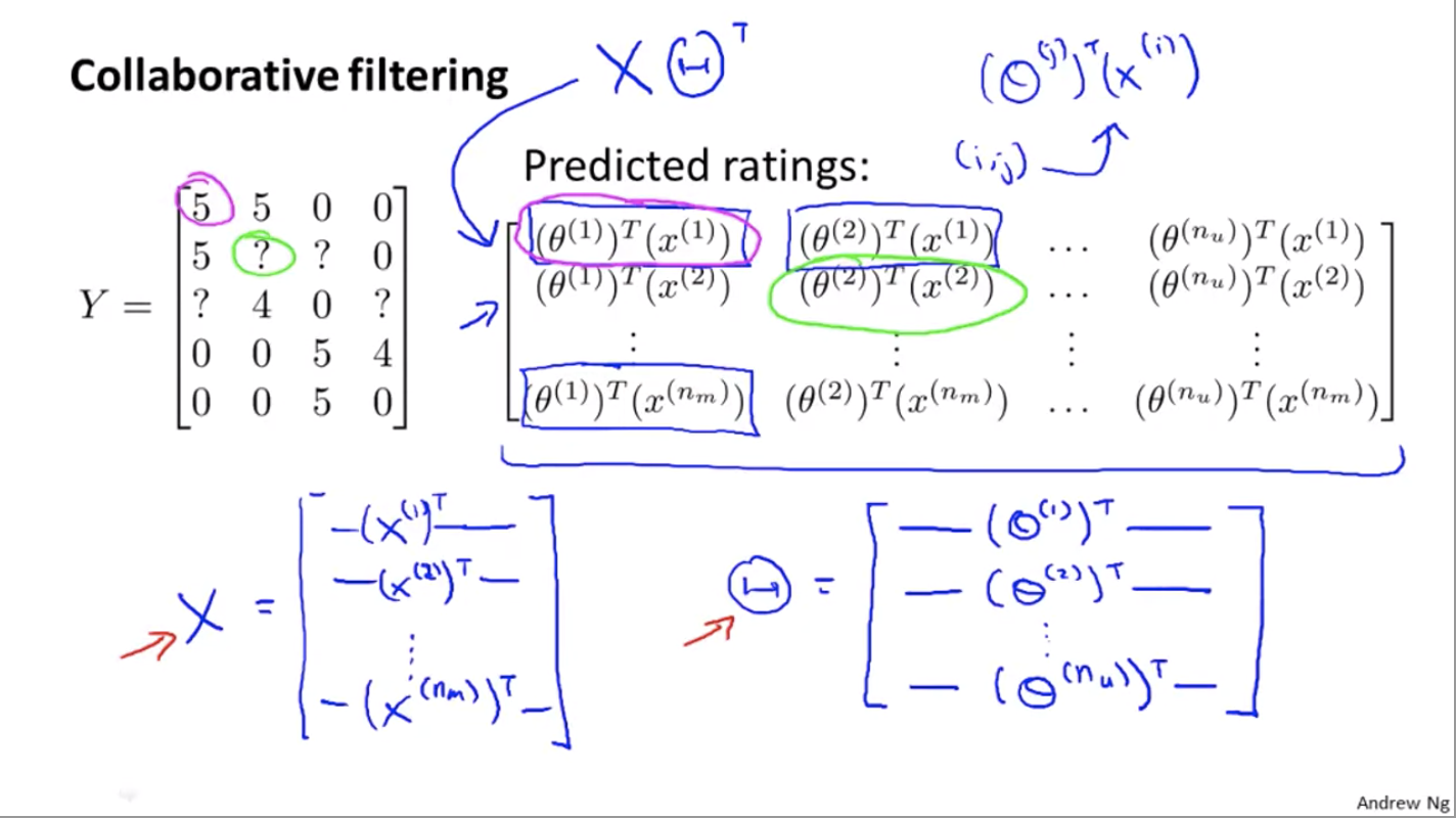
Vectorization

The matrix in the top right corner equals to$X\Theta^T$.

Application: Similar Movies

Let’s say movie $i$’s features is $x^{(i)}$. How can we find a movie $j$ that is similar to the movie $i$?

We can do so by finding a movie with features $x^{(j)}$ such that $||x^{(i)} - x^{(j)}||$ is small.

What if there is a user that hasn’t given any rating to any movie?

If we go to the cost function above, the first term will be gone since none of $r(i, j) = 1$ for that user (they didn’t give any rating). So what we try to minimize will be $\frac{\lambda}{2} \sum{j=1}^{n_u} \sum{k = 1}^n(\theta_k^{(j)})^2$, which will give us $\theta = 0$.

But it doesn’t make sense to say that this user dislikes all movies.

So rather than giving all zeros, let’s assume the user’s rating for a movie is the average rating of that movie from other users who rated that movie.

Week 10 - Large Scale Machine Learning

“In machine learning, it’s not who has the best algorithm that wins. It’s who has the most data.”

A problem with learning with large datasets is that recall for gradient descent, we have a summation from 1 to m where m is the size of the dataset. So for each gradient descent, we’ll need to run the summation over the entire dataset, which is very inefficient.

How can we know if a dataset is big enough? Or should we add more data to it to get a better training result?

The answer is: learning curves! (week 6)

Plot a learning curve and see whether it’s a high variance or a high bias. If high variance, then increasing the data size will give us a better result, while if it’s a high bias, increasing the data size won’t help.

Stochastic Gradient Descent

As stated above, when the data size is large, our old gradient descent (batch gradient descent) will be very expensive to calculate. To scale the algorithm for larger datasets, we’ll use stochastic gradient descent.

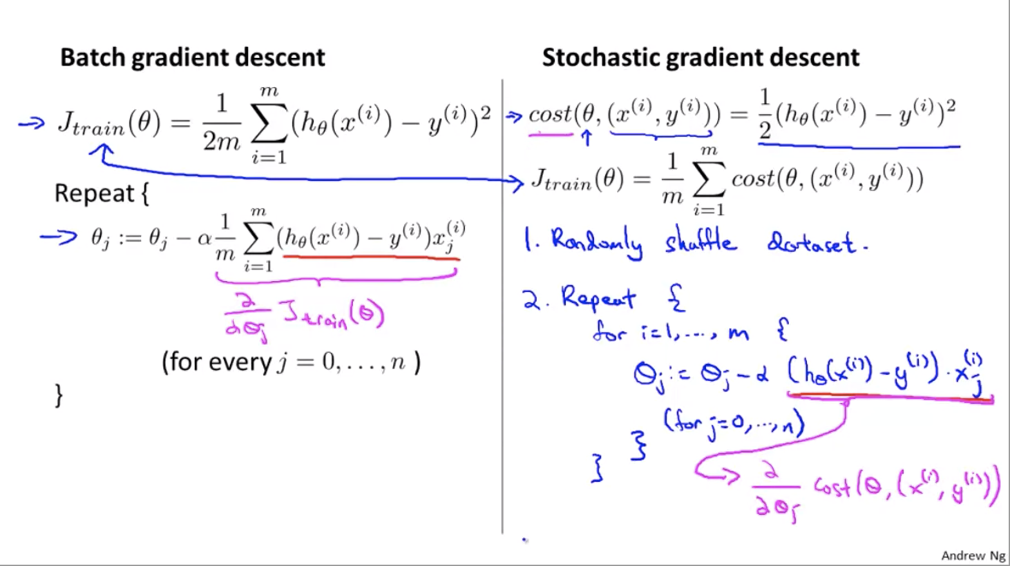
Note that we no longer have that summation in the equation. We improve each $(x^{(i)}, y^{(i)})$ only on its old value, rather than waiting for the summation to get all the old values.

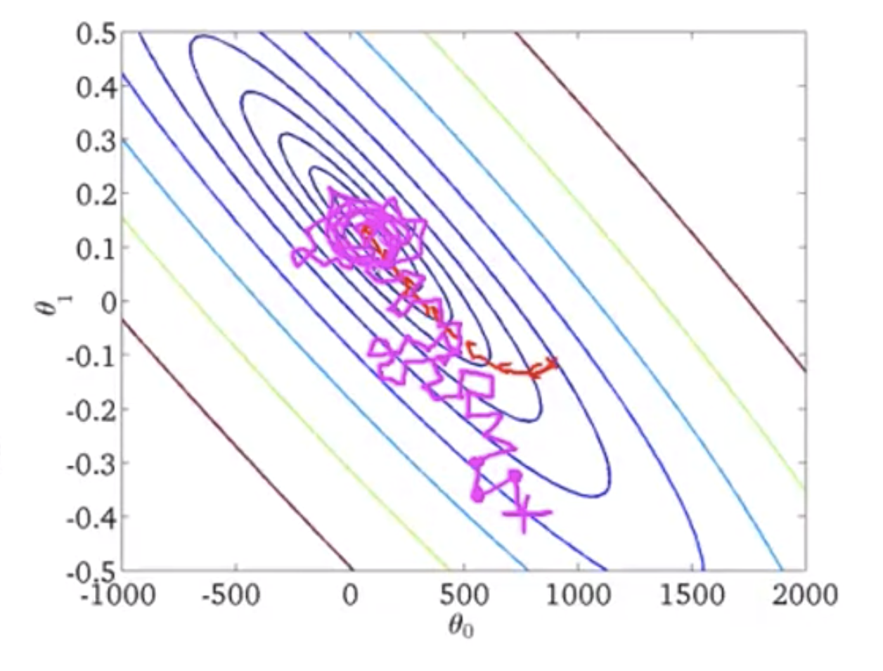
In the figure below:

• red is for batch gradient descent: always moves to a better value
• pink is for stochastic gradient descent: takes more steps since each iteration is faster, but not every step is a good direction

Mini-batch Gradient Descent

• Batch gradient descent: use all $m$ examples in each iteration
• Stochastic gradient descent: use 1 examples in each iteration
• Mini-batch gradient descent: use $b$ examples in each iteration ($b$ is up to our choice, usually from 2 to 100)

e.g. when $b = 10$:

$$\theta_j := \theta_j - \alpha \frac{1}{10}\sum_{i=k}^{k+9} (h(x^{(i)}) - y^{(i)})x_j^{(i)}$$

And in each iteration, increase $k$ by 10.

Checking for Convergence

When doing batch gradient descent, we can make sure that the function converges by looking at the cost function — it should be non-increasing.

How can we check for stochastic gradient descent?
The answer is to compute $cost(\theta, (x^{(i)}, y^{(i)}))$ before updating $\theta$ using $(x^{(i)}, y^{(i)})$. And for every, say, 1000 iterations, plot the average cost of the last 1000 iterations and see how well the algorithm runs.

Usually, stochastic gradient descent ends up in a place that is close to the global minimus (but not exactly the global minimum). If we want stochastic gradient descent to actually converge to the global minimum, we can slowly decrease the learning rate alpha over time: $\alpha = \frac{\text{const1}}{\text{iterationNumber + const2}}$.

But people usually don’t do this, because it requires some tuning on the constants. But if we can tune it well, we will reach the global minimum.

Online Learning

Let this code run forever on the server:

$$\text{get } (x, y )\text{ from the user and update } \theta \text{ using } (x, y):\\ \theta_j := \theta_j - \alpha (h(x) - y)x_j \;\;\forall j = 1, \ldots, n\\ \text{after that, we can discard } (x, y)$$

If many users keep arriving at the website, we’ll have enough data for training. And this is very adaptive e.g. when the trend changes, $\theta$ can correspond to the change because of tons of updated data from the users.

Week 11 - Photo OCR

Photo OCR Pipeline

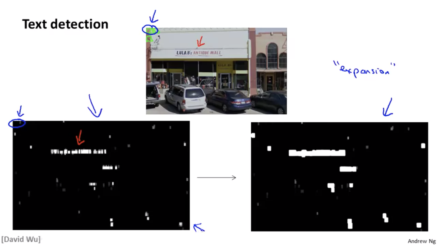
1. Text detection: find the text regions on the photo
2. Character segmentation: segment the text into individual chars
3. Character classification

Sliding Window

e.g. pedestrian detection

1. Train some sample patches of size $w * h$
2. Slide a frame of size $w * h$ through the photo, see if the segment in the frame is positive/negative
3. Slide the frame by step size (the smaller the better, but also more computationally expensive)
4. Resize the frame to a bigger/smaller size, repeat the steps above (because the size of pedestrians in the photo are different depending on how close/far they are)

Text Detection

We’ll run the sliding window algorithm and find the characters, then “expand” the text region.

How to know where to split the character?

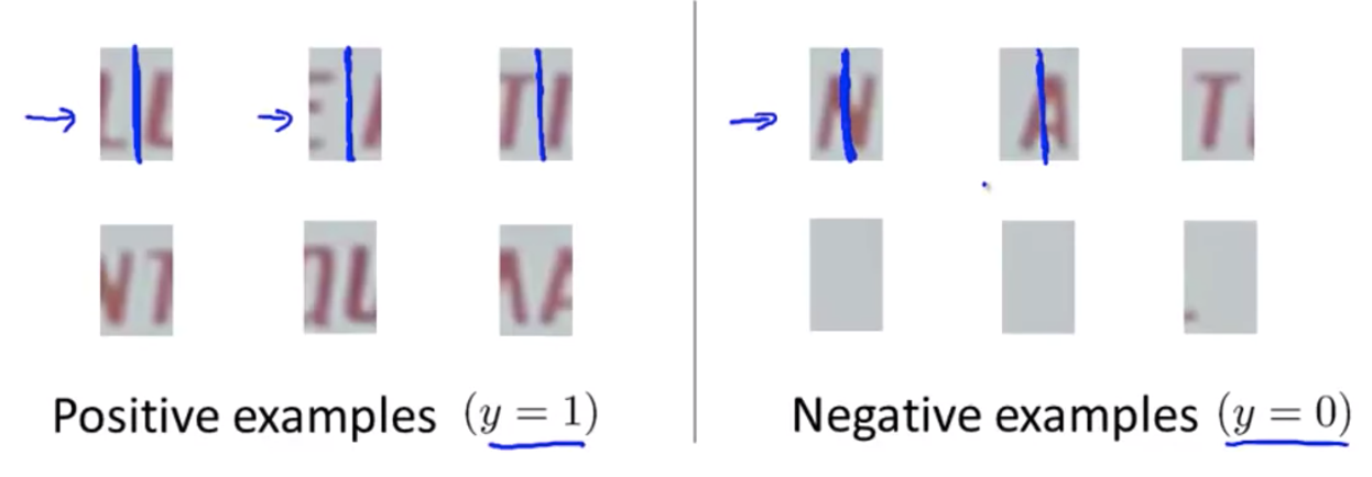
Look for a blank line in the middle between two chars.

Artificial Data Synthesis

If the number of training data is not enough, we can synthesize data. But before we do that, let’s consider the following:

1. Make sure we have a low bias classifier before synthesizing more data. If the classifier is of high bias, increasing the number of training data wouldn’t help.
2. How much work will it take to synthesize 10x more data?

What Part of the Pipeline to Work on Next？

Use Celling Analysis.

Let’s say we have a pipeline:

Step 1 —-> Step 2 —-> Step 3

1. Check the overall accuracy of the pipeline: 72%
2. Instead of using the output from Step 1, manually give Step 2 100% accurate data as input, and the accuracy of the entire pipeline is now 89%
3. Instead of using the output from Step 2, manually give Step 3 100% accurate data as input, and the accuracy of the entire pipeline is now 99%

So we know that: if we improve Step 1‘s accuracy, the overall accuracy goes up by 17%, and if we improve Step 2‘s accuracy, the overall accuracy goes up by 10%, etc.

Therefore, we should put more effort into Step 1.